Probability mass functions

Definition

Probability Mass Function (PMF):

  • denoted by \(p\) (not to be confused by \(\mathbb{P}\)),
  • defined by: \[p(x) = \mathbb{P}(X = x).\]
  • Terminology: \(\{x : p(x) > 0\}\) is called the support.
  • If there are several random variables, we use a subscript to disambiguate the PMFS, e.g.,
    • \(p_X\) for the PMF of the latent random variable,
    • \(p_Y\) for the PMF of the observed random variable.

Example: coins

  • PMF of fair coin: \(p(0) = p(1) = 1/2\)
  • Generalization: the family of Bernoulli PMFs
  • Recall: when you flip a “Biased” coin
    • get a 1 with probability \(p \in [0, 1]\)
    • get a 0 with probability \(1 - p\)
  • \(p\) is an example of what is called a PMF’s parameter
  • Notation: \(X \sim {\mathrm{Bern}}(p)\)

Example: discrete uniform distributions

  • Example: dice
  • Notation: \(Y \sim {\mathrm{Unif}}\{1, 2, 3, 4, 5, 6\}\)

Simulation/sampling from a PMF

In R

require(extraDistr)
Loading required package: extraDistr
# 10 coin flips:
rbern(10, prob=0.5)
 [1] 1 1 0 1 1 0 0 0 1 1
# two dice rolls
rdunif(2, min=1, max=6)
[1] 3 6

How does it work?

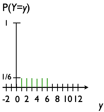
  • Think of the green lines in the uniform PMF as “sticks” with “labels.”
    • The “labels” are the different realization, e.g. 1, 2, 3, …, 6.
  • Place the six sticks in the interval \([0, 1]\) so that they do not overlap.
  • Sample a uniform real number in \([0, 1]\)
    • in R: runif(1)
  • The uniform falls in exactly one of the sticks.
  • Return the label of that stick.

Mathematical explanation

The above “stick-based” algorithm can be implemented using the cumulative distribution function and a generalization of its inverse known as the quantile function.

Cumulative distribution function (CDF): \(F(x) = \mathbb{P}(X \le x).\)

Quantile function: \(Q(u) = \inf\{x \in \mathbb{R}: u \le F(x)\}\).

Then the “stick-based” algorithm can be written as:

  1. \(U \sim {\mathrm{Unif}}[0, 1]\)
  2. Return \(Q(U)\).

Plotting PMFs in R

Here is an example of how to plot PMFs in R:

realizations <- 0:20

plot(realizations, dbinom(realizations, size=20, prob=.3), type='h')

Some explanations:

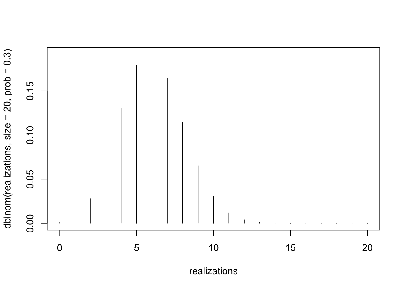
  • Here dbinom is the R function for the PMF of a binomial (R uses the prefix d___ for densities and PMFs).
  • We use the fact that many functions in R such as this one are vectorized, i.e. the normal PMF function takes a single point \(x\) and output \(p(x)\) where \(p\) is the PMF; the vectorized version takes vector \((x_1, x_2, \dots)\) and returns \((p(x_1), p(x_2), \dots)\).
  • The argument type = 'h' instructs the plot function to make the plot “histogram”-like.