Importance sampling

Outline

Topics

• What Self-Normalizing Importance Sampling (SNIS) does.
• Intuition on how SNIS does it.
• SNIS pseudo-code.

Rationale

Since SNIS is the “inference algorithm” used by simPPLe, you will need a basic understanding of SNIS to complete this week’s exercise.

Goal

• Our goal is to compute \(\mathbb{E}[g(X) | Y = y]\).
• SNIS will allow us to approximate this conditional expectation.

How is this different than the simple Monte Carlo method that we used in Ex1.Q.1.3?

Click for answer

We used simple Monte Carlo to compute an expectation without conditioning on \(Y = y\), i.e. \(\mathbb{E}[g(X)]\).

SNIS allows us to take into account observed data.

Problem formulation

SNIS is used to solve the following type of problems:

• Input: You are given an unnormalized distribution \(\gamma(x)\)
  • Example: the numerator in Bayes rule.
• Output: You want to approximate an expectation…
  • …under the renormalized distribution \(\pi(x) = \gamma(x) / Z\).
  • Mathematically: SNIS provides an approximation to \(\mathbb{E}_\pi[g(X)] = \sum \pi(x) g(x)\).

Terminology: \(g\) is called a test function. Think about it as specifying a query.

Examples: of test functions

• Let’s say you want to approximate \(\mathbb{P}(X = 1 | Y = y)\).
  • We can do this with SNIS by picking the right \(g\)!
  • From last week’s “trick 2”, if we take \(g(x) = \mathbb{1}[X = 1]\), \(\pi(x) = p(x | y)\), \[\mathbb{E}_\pi[g(X)] = \sum \pi(x) g(x) = \mathbb{E}[\mathbb{1}[X = 1] | Y = y] = \mathbb{P}(X = 1 | Y = y).\]
• What function \(g(x)\) would you take to compute a posterior mean?

Click for choices

1. \(g(x) = \mathbb{1}[X = x]\)
2. \(g(x) = \mathbb{1}[x]\)
3. \(g(x) = x\)
4. \(g(x) = x^2\)
5. None of the above

Click for answer

If we set \(g(x) = x\), then \(\sum x \pi(x) = \mathbb{E}[X | Y = y]\).

• How would you proceed to compute \(\operatorname{Var}[X | Y = y]\)?

SNIS’ extra ingredient: the proposal

In addition to the unnormalized distribution \(\gamma\) and test function \(f\), SNIS requires a proposal \(q(x)\).

• The proposal will help SNIS explore the space of possible values that \(X\) can take.
• This week, we will use the prior as the proposal, \(q(x) = \rho(x)\).
  • It can be generalized to any PMF \(q(x)\) such that \(q(x) = 0 \Longrightarrow \pi(x) = 0\).

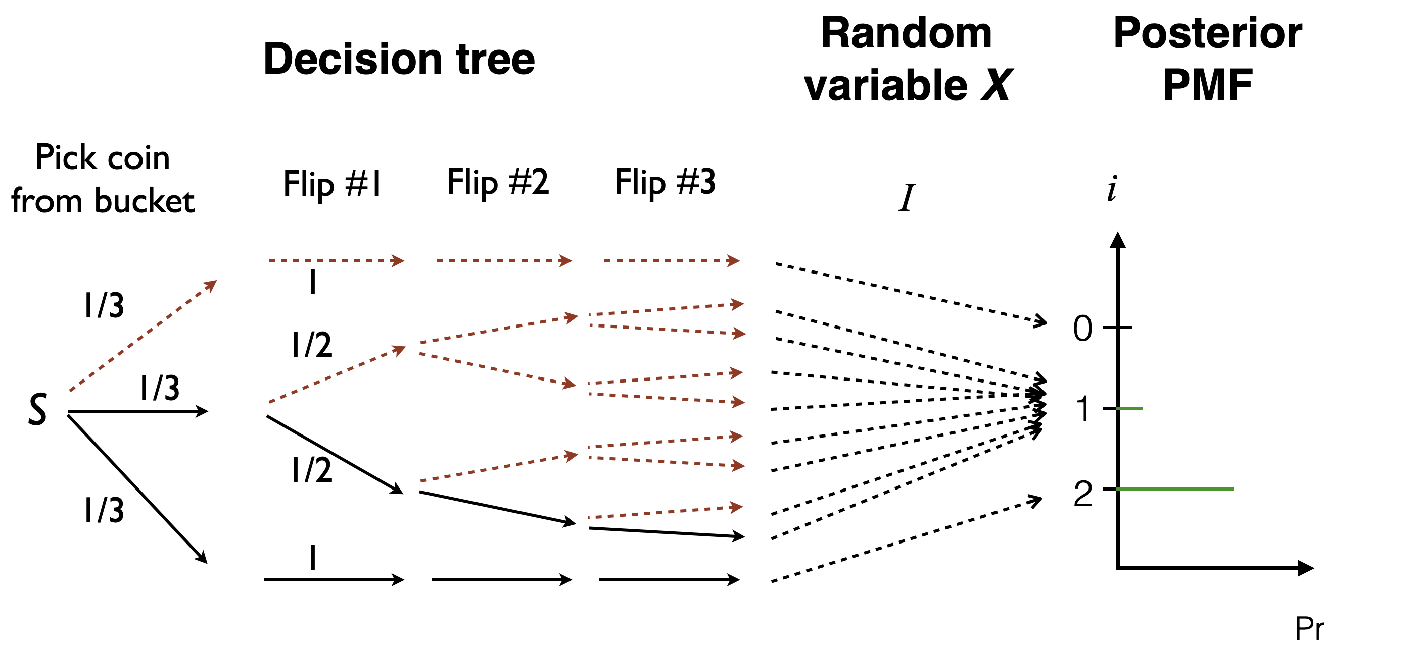
Intuition: decision tree

• Recall the forward_sample function from the first exercise, Q.1.3.
• SNIS follows the same general approach (Monte Carlo),
  • traverse the decision tree several times to get “samples”
  • the key difference is that these samples will not be equally weighted in SNIS in contrast to Q.1.3.
• At each iteration, just as forward sampling, SNIS goes down the decision tree…
  • …but for some decision points, the choice is made for us—by the data!
    • Call these “forced choices.”
  • We keep track of the probability of the “forced choices”,
    • the product of these probability will be the un-normalized weight of the sample.

Algorithm

• Call the proposal \(M\) times.
  • Denote the output at iteration \(m \in \{1, 2, \dots M\}\) by: \[(X^{(m)}) \sim q(\cdot)\]
  • Compute \(g\) on each, call each of the \(M\) outputs \(G^{(m)}\) \[G^{(m)}= g(X^{(m)}).\]
  • Compute also an un-normalized weight for each of the \(M\) outputs: \[W^{(m)}= w(X^{(m)}) = \frac{\gamma(X^{(m)})}{q(X^{(m)})}.\] - Here \(w(x)\) is a weighing function.
• Return the ratio \[\hat G_M = \frac{\sum_{m=1}^M W^{(m)}G^{(m)}}{\sum_{m=1}^M W^{(m)}} .\]

Example: compute \(\hat G_M\) in the bag of coin example if \(g(x) = x\), \(X^{(1)} = 1\), \(X^{(2)} = 2\). Use the decision tree above to help you.

Click for choices

1. \(0\)
2. \(1.5\)
3. \(\approx 1.89\)
4. \(\approx 2.17\)
5. None of the above

Click for answer

We have:

\(m\)	\(X^{(m)}\)	\(W^{(m)}\)	\(W^{(m)}G^{(m)}\)
1	1	\((1/2)^3\)	\((1/2)^3\)
2	2	1	2

Hence:

\[\hat G_M = \frac{(1/2)^3 + 2}{(1/2)^3 + 1} \approx 1.89.\]

Weight simplification

• Recall from chain rule: \(\gamma(x) = p(x, y) = \rho(x) L(y | x)\) where \(\rho\) is the prior and \(L\) the likelihood.
• Hence, since the proposal is the prior \(q(x) = p(x)\), the weight calculation simplifies to \[w(x) = \frac{\gamma(x)}{q(x)} = \frac{\rho(x) L(y | x)}{\rho(x)} = L(y | x).\]

Theoretical guarantees of SNIS

• We have the same type of result as we encountered in Simple Monte Carlo
• Namely: for any approximation error tolerance, we can find a number of iterations \(M\) large enough such that we will be within that error tolerance with high probability after \(M\) iterations.
• Name for the above property: consistency.

Proposition: if \(\mathbb{E}_\pi|g(X)| < \infty\), then¹ \[\hat G_M \to \mathbb{E}_\pi[g(X)],\] as \(M\) goes to \(\infty\).

Further readings

• Art Owen’s notes, available form the author’s website
• Chopin and Papaspiliopoulos, Chapter 8 [Available online via UBC Library]

Footnotes

1. Here “\(\to\)” can be taken to be “convergence in probability”, or this can be strengthen to “convergence almost sure.”