Grouped data

Outline

Topics

• Using the package tidybayes to feed complex data into Stan.

Rationale

Data organized in various groups is a frequent feature of Bayesian models, in particular in hierarchical models.

Getting grouped data into stan is tedious and error-prone. The package tidybayes automates much of this.

Pre-reading

If you have never heard about “tidy data”, while it is not strictly essential for this course, it is a good investment to skim this tutorial on tidy data.

Example

First, install the packages magrittr and tidybayes (and ggplot2 if you have not done so already), then import them:

suppressPackageStartupMessages(library(cmdstanr))
suppressPackageStartupMessages(library(magrittr))
suppressPackageStartupMessages(library(tidybayes))
suppressPackageStartupMessages(library(ggplot2))

Data prep

We load data modelling covid vaccines efficacy:

data = read.csv(url("https://raw.githubusercontent.com/UBC-Stat-ML/web447/main/exercises/ex06_assets/vaccines_full.csv"))
data$is_vaccinated = ifelse(data$arms == "vaccinated", 1, 0)
rmarkdown::paged_table(data)

The magic conversion of “tidy data” (data in a format like the above) into a format that can be consumed by Stan is done using compose_data:

stan_converted = compose_data(data)

stan_converted

$trials
[1] 1 1 3 3 2 2

$n_trials
[1] 3

$arms
[1] 2 1 2 1 2 1

$n_arms
[1] 2

$groupSizes
[1]  5807  5829 18198 18325 14134 14073

$numbersOfCases
[1]  30 101   8 162  11 185

$is_vaccinated
[1] 1 0 1 0 1 0

$n
[1] 6

Stan model

Here we consider a simple, non-hierarchical model but fitting all the data at once. As an exercise, think about how you can modify this model to be hierarchical.

vaccines.stan

data {
  int n;
  int n_trials;
  array[n] int<lower=1,upper=n_trials> trials;
  array[n] int arms;
  int n_arms;
  array[n] int groupSizes;
  array[n] int numbersOfCases;
  array[n] int is_vaccinated;
}

parameters {
  vector<lower=0,upper=1>[n_trials] efficiencies;
  vector<lower=0,upper=1>[n_trials] prevalences;
}

model {

  for (trial in 1:n_trials) {
    efficiencies[trial] ~ beta(1, 1);
    prevalences[trial] ~ beta(1, 1);
  }

  for (i in 1:n) {
    numbersOfCases[i] ~ binomial(groupSizes[i], prevalences[trials[i]] * (is_vaccinated[i] == 1 ? 1.0 - efficiencies[trials[i]] : 1.0));
  }
}

Fitting

The fit object returned by sample() does not know about the string labels attached to each trial integer index. We use fit %<>% recover_types(data) to add back that information:

mod = cmdstan_model("vaccines.stan")
fit = mod$sample(
  seed = 1,
  data = stan_converted, 
  output_dir = "stan_out",
  refresh = 0,
  iter_sampling = 10000                  
)
fit %<>% recover_types(data)

Getting draws

The output of Stan is not tidy either.

fit

        variable     mean   median   sd  mad       q5      q95 rhat ess_bulk
 lp__            -2793.20 -2792.87 1.74 1.58 -2796.52 -2790.99 1.00    18550
 efficiencies[1]     0.69     0.69 0.06 0.06     0.57     0.78 1.00    47395
 efficiencies[2]     0.93     0.94 0.02 0.02     0.90     0.96 1.00    52259
 efficiencies[3]     0.94     0.95 0.02 0.02     0.91     0.97 1.00    48810
 prevalences[1]      0.02     0.02 0.00 0.00     0.01     0.02 1.00    44590
 prevalences[2]      0.01     0.01 0.00 0.00     0.01     0.01 1.00    51935
 prevalences[3]      0.01     0.01 0.00 0.00     0.01     0.01 1.00    51276
 ess_tail
    26750
    29969
    30050
    28217
    30768
    29448
    30109

Use spread_draws to put the draws into a tidy format:

fit %>% spread_draws(efficiencies[trials], prevalences[trials]) %>% head(10)

# A tibble: 10 × 6
# Groups:   trials [1]
   trials               efficiencies .chain .iteration .draw prevalences
   <chr>                       <dbl>  <int>      <int> <int>       <dbl>
 1 AZ-Oxford (combined)        0.656      1          1     1      0.0153
 2 AZ-Oxford (combined)        0.626      1          2     2      0.0169
 3 AZ-Oxford (combined)        0.739      1          3     3      0.0168
 4 AZ-Oxford (combined)        0.731      1          4     4      0.0160
 5 AZ-Oxford (combined)        0.768      1          5     5      0.0189
 6 AZ-Oxford (combined)        0.552      1          6     6      0.0158
 7 AZ-Oxford (combined)        0.608      1          7     7      0.0164
 8 AZ-Oxford (combined)        0.695      1          8     8      0.0188
 9 AZ-Oxford (combined)        0.809      1          9     9      0.0195
10 AZ-Oxford (combined)        0.755      1         10    10      0.0184

Plotting

Now that we have draws in tidy format, instead of using specialized MCMC plotting libraries we can just use ggplot:

fit %>%
  spread_draws(efficiencies[trials]) %>%
  ggplot(aes(x = efficiencies, y = trials)) +
  stat_halfeye() + 
  theme_minimal()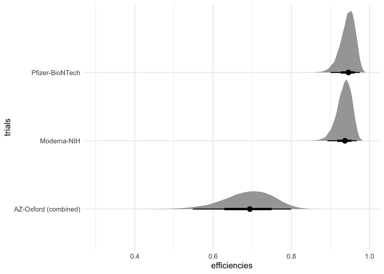

This makes it easier to customize plots.

Summaries

tidybayes also offers convenient ways to compute summaries such as High Density Intervals (HDI)

fit %>%
  spread_draws(efficiencies[trials]) %>%
  median_hdi(efficiencies)

# A tibble: 3 × 7
  trials               efficiencies .lower .upper .width .point .interval
  <chr>                       <dbl>  <dbl>  <dbl>  <dbl> <chr>  <chr>    
1 AZ-Oxford (combined)        0.694  0.558  0.806   0.95 median hdi      
2 Moderna-NIH                 0.937  0.897  0.970   0.95 median hdi      
3 Pfizer-BioNTech             0.946  0.905  0.978   0.95 median hdi      

More information

See the tidybayes documentation.