Variational methods
Outline
Topics
- Variational approximations
- Distribution families
- Posterior approximation as optimization
Rationale
In certain situations, and for a finite time budget, variational methods can provide a better approximation than MCMC methods.
What is a variational method?
Setup: as in MCMC…
- we try to approximate a posterior \(\pi(x)\) with \(x \in \mathscr{X}\),
- known only up to normalization constant, \(\pi(x) = \gamma(x) / Z\).
Additional ingredient: a family (set) of distributions, \(\mathscr{Q}= \{q_\phi : \phi \in \Phi\}\) called the variational family.1
- Each element of the variational family is a density/PMF \(q_\phi(x)\) defined on the same space as \(\pi(x)\).
- Each element is indexed by a variational parameter \(\phi \in \Phi\).
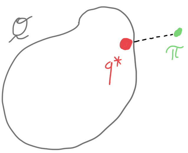
Variational inference: find a variational approximation \(q^*_\phi\in\mathscr{Q}\) as close as possible to the posterior \(\pi\).
Distribution families
Example: consider the beta-binomial example.
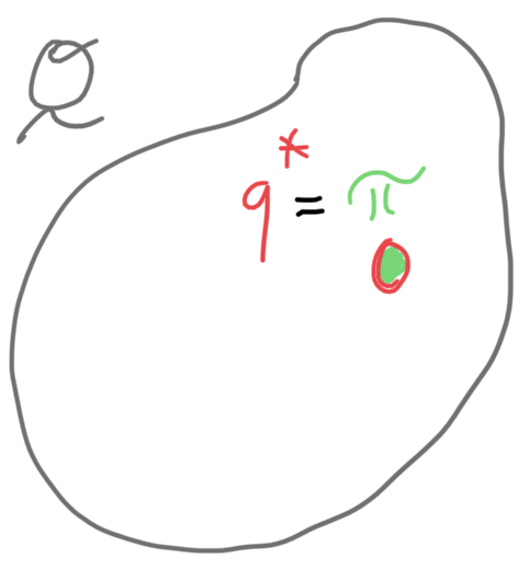
- Here we could take \(\mathscr{Q}\) to be the set of all beta distributions.
- The beta family has two positive parameters, \(\phi = (\alpha, \beta)\), \(\alpha, \beta > 0\)…
- … so \(\Phi = \mathbb{R}^+ \times \mathbb{R}^+\).
- This is the “best case” for variational inference:
- from a practice quiz exercise, \(\pi \in \mathscr{Q}\),
- so \(q^*_\phi = \pi\), i.e., variational inference incurs no approximation error in this special case (see figure).
- Typically, we do not have tractable (easy to compute) conjugate family though.
Example: when \(\mathscr{X}= \mathbb{R}\), a typical choice of variational family is to use a normal family.
Question: for the normal variational family, complete the definition of variational approximation \(q_\phi\), variational parameter \(\phi\) and parameters \(\Phi\).
- \(q_\phi(x) = \exp(-(x - \mu)^2 /(2\sigma^2))\), \(\phi = (x, \mu, \sigma^2)\), \(\Phi = \mathbb{R}\times \mathbb{R}\times \mathbb{R}^+\).
- \(q_\phi(x) = \exp(-(x - \mu)^2 /(2\sigma^2))\), \(\phi = (\mu, \sigma^2)\), \(\Phi = \mathbb{R}\times \mathbb{R}^+\).
- \(q_\phi(x) = (\sigma \sqrt{2\pi})^{-1} \exp(-(x - \mu)^2 /(2\sigma^2))\), \(\phi = (x, \mu, \sigma^2)\), \(\Phi = \mathbb{R}\times \mathbb{R}\times \mathbb{R}^+\).
- \(q_\phi(x) = (\sigma \sqrt{2\pi})^{-1} \exp(-(x - \mu)^2 /(2\sigma^2))\), \(\phi = (\mu, \sigma^2)\), \(\Phi = \mathbb{R}\times \mathbb{R}^+\).
- None of the above.
Correct answer is 4: in this example…
- Each distribution in the family is a normal density, \(q_\phi(x) = (\sigma \sqrt{2\pi})^{-1} \exp(-(x - \mu)^2 /(2\sigma^2))\).
- Notice we need to incorporate the normalization constant of \(q\), this will be important in our calculations later on.
- A variational parameter here is a mean and a variance, \(\phi = (\mu, \sigma^2)\).
- Hence the variational parameters are \(\Phi = \mathbb{R}\times \mathbb{R}^+\).
Footnotes
Notice we also used \(q\) for MCMC proposal and importance sampling’s importance distribution. These are different but related. It is a general convention to use \(q\) for “quantities that help us to approximate a complex distribution.” The connection between variational inference’s \(q\) and importance sampling’s \(q\) is more direct compared to MCMC’s proposal \(q\).↩︎