Stan: going further

Outline

Topics

• More complex types in Stan (vectors, constraints)
• Loops and vectorization
• Feeding complex data into Stan

Rationale

We review here the constructs needed to write more complex models such as the exercises coming in the next few weeks, and the second quiz.

Example

The data below consists, for each day in December 2021, of the percentage of sequenced COVID-19 samples that are of the Omicron variant.

suppressPackageStartupMessages(library(cmdstanr))
suppressPackageStartupMessages(library(ggplot2))
suppressPackageStartupMessages(library(dplyr))

# data from: https://data.chhs.ca.gov/dataset/covid-19-variant-data
df = read.csv("../data/covid19_variants.csv")
df$date = as.Date(df$date,format="%Y-%m-%d")

df = df %>% filter(date > "2021-12-01" & date < "2021-12-31") %>% filter(variant_name == "Omicron")

df %>% ggplot(aes(x = date, y = percentage)) + geom_point() + ylim(0, 100) + theme_minimal()

Model (mathematical notation)

One possible model for this data: for \(i \in \{1, 2, \dots, N\}\), \(N\) being the number of days in December (\(N=31\)),¹

\[\begin{align*} \theta_0 &\sim {\mathrm{Exp}}(1) \\ \theta_1 &\sim \mathcal{N}(0, \sigma = 1000) \\ \theta_2 &\sim \mathcal{N}(0, \sigma = 1000) \\ \mu_i &= \text{logistic}(\theta_1 (i/N) + \theta_2) \\ y_i &\sim {\mathrm{Beta}}(\mu_i, \theta_0) \\ \end{align*}\]

Model (in Stan)

Let us translate the mathematical notation into Stan:

omicron_first_attempt.stan

// comments in Stan use '//' not '#'

data { 
  // Here `N` is the number of days considered. 
  int N; 
  
  // meaning: `y` is a vector of length `N` where each entry is between zero and one.
  vector<lower=0, upper=1>[N] y; 
}

// As before, we declare in `parameters` the types of the unobserved (latent) random variables. 
parameters { 
  real<lower=0> concentration; 
  real slope;
  real intercept;
}

model {
  concentration ~ exponential(1);
  slope ~ normal(0, 1000);
  intercept ~ normal(0, 1000);
  
  for (i in 1:N) { // Stan is 1-indexed
    // inv_logit is Stan's name for the logistic function
1    y[i] ~ beta_proportion( //
              inv_logit(intercept + slope * (i/N)), 
              concentration); 
  }
}

1

Here, beta_proportion corresponds to the mean-concentration parameterization we discussed in the lecture on hierarchical models.

Question: how do you think Stan will use the parameters’ type constraints? (e.g., <lower=0> in real<lower=0> concentration)?

Click for choices

1. To validate input data
2. To validate MCMC initialization
3. To perform a change of variable
4. To perform a change of variable and validate input data
5. To perform a change of variable and validate MCMC initialization

Click for answer

Correct answer is to perform a change of variable and validate MCMC initialization.

In Stan, we use a version of HMC that works best when the state space to be unconstrained. So internally Stan will get rid of the constraints using a transform suited for each type of constraints offered in the Stan language.

What about the Jacobian involved in the change of variable? Stan will compute that for you using automatic differentiation. Much less painful than when we did it manually for the Laplace approximation!

Improving our model with transformed parameters

• The code in the last section will not print out \(\mu_i\)
• The code below shows how to fix this
  • \(\mu_i\) is handled differently than \(\theta_k\), \(y_i\)…
  • … because \(\mu_i\) is defined with \(=\) instead of \(\sim\)

omicron.stan

data { 
  int N; 
  vector<lower=0, upper=1>[N] y; 
}

parameters { 
  real<lower=0> concentration; 
  real slope;
  real intercept;
}

1transformed parameters { //
  // linspaced_vector(N,0,1) creates a vector 
  //    of N equispace points between 0 and 1
  //    (we normalize the dates to be between zero and one)
  // functions in Stan are typically vectorized, 
  //    this is the case for example with inv_logit
  vector[N] mu = 
    inv_logit(intercept + slope*linspaced_vector(N,0,1));
}

2model { //
  concentration ~ exponential(1);
  slope ~ normal(0, 1000);
  intercept ~ normal(0, 1000);
  
  // Another example of vectorization---the line below will produce the same 
  // output as the loop in the previous version, but slightly faster:
  y ~ beta_proportion(mu, concentration);
}

1

Whenever in the mathematical notation a latent random variable is defined using an equality (“\(=\)”), and you want to have it as part of the output, write it in the transformed parameters block.

2

Whenever in the mathematical notation a latent random variable is defined using a distribution statement (“\(\sim\)”), write it in the model block.

Running MCMC

Running MCMC on the model is done as before:²

data_without_zeros = pmax(pmin(df$percentage/100,0.999),0.001)

mod = cmdstan_model("omicron.stan")
fit = mod$sample(
1  data = list(
          y = data_without_zeros, 
          N = length(data_without_zeros)
        ), 
2  chains = 1,
  iter_sampling = 10000,
  refresh = 5000,
  output_dir = "stan_out",
)

1

Each variable in Stan’s data block needs to be fed a value when called from R.

2

The chains option can be used to simulate several independent MCMC chains, moreover, they can be sampled in parallel using instead parallel_chains in mod$sample(...).

Running MCMC with 1 chain...

Chain 1 Iteration:     1 / 11000 [  0%]  (Warmup) 
Chain 1 Iteration:  1001 / 11000 [  9%]  (Sampling) 
Chain 1 Iteration:  6000 / 11000 [ 54%]  (Sampling) 
Chain 1 Iteration: 11000 / 11000 [100%]  (Sampling) 
Chain 1 finished in 0.4 seconds.

Posterior visualization

We can extract samples as follows:

samples = posterior::as_draws_matrix(fit$draws("mu"))
n_samples = nrow(samples)
n_samples

[1] 10000

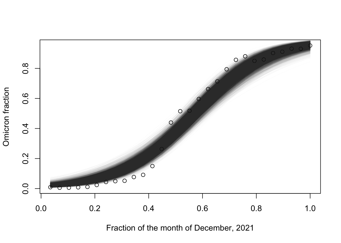
and plot the posterior distribution over the beta’s mean functions:

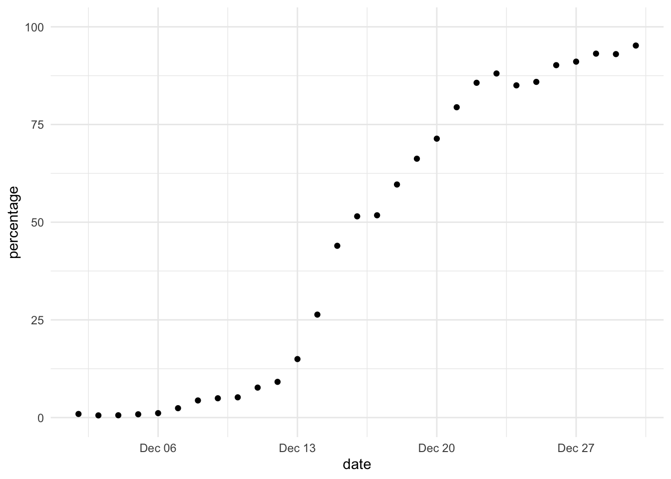
data = df$percentage
xs = 1:length(data) / length(data)

plot(xs, data/100, 
      xlab = "Fraction of the month of December, 2021", 
      ylab = "Omicron fraction")

for (i in 1:n_samples) {
  lines(xs, samples[i,], col = rgb(red = 0, green = 0, blue = 0, alpha = 0.01))
}

Model criticism

What are potential weakness(es) of the model?

Click for answer

Many answers possible. For example, the systematic errors in the residuals (i.e., many points in a row are smaller at the beginning, and the reversed trend at the end) suggest that the logistic function is not quite rich enough to capture the details of the observed curve.

Footnotes

1. In the model below, notice we normalize the day by \(N\) to put it in the interval \([0, 1]\). This is not strictly necessary, but often, bringing covariates into a nice range can make sampling faster when it reduces the condition number of the sampling problem.

2. note that we make sure no datapoints have value zero or one as under certain parameter values of the beta distribution, this can lead to a zero density point which Stan is not able to handle.