(Normal) regression

Outline

Topics

A second example of a Bayesian model based on a linear model, this time with a normal likelihood.
Priors on the positive real line.
Homoscedasticity and heteroscedasticity.
Marginal posterior.

Rationale

Together with classification (previous page), regression is the other major statistical task frequently encountered.

We see here that the same approach as we took for classification can be easily modified to do regression.

This provides us with a second example of Bayesian GLMs.

Example

In the early 20th century, astronomers made the startling observation that pretty much all galaxies are moving away from ours. Why?
We now know this is because the universe is expanding.
Here is a metaphor to help understand this:
- Imagine ants on an inflating balloon.
- You are one of the ants…
- …and you notice that all the others ants are moving away from you…
  - …and the further the neighbor ant, the faster it looks like it is moving away from you.
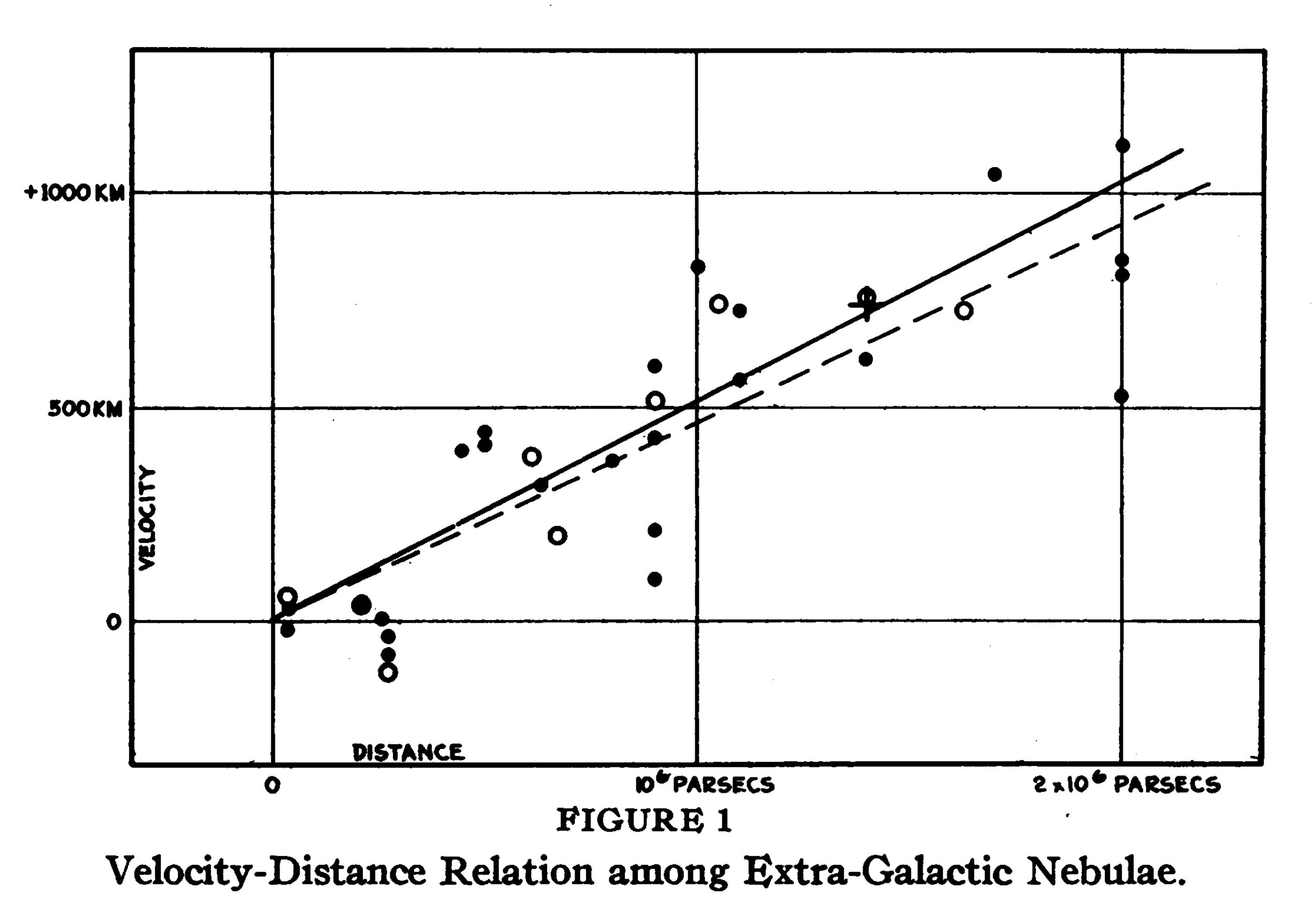
In 1929 the astronomer Edwin Hubble published a paper¹ on the relationship between distance and velocity of galaxies relative to us.
It is now called Hubble’s law.
The estimated slope of the relationship, known as Hubble’s constant, leads to an estimate of the age of the universe.

Data

We will estimate Hubble’s constant using data from the original data used by Edwin Hubble (in CSV).
To make the numbers less extreme in the following, I will divide the velocities by 1000

Instructions:

download the CVS
copy paste the code below and run it on your computer (after changing the path “../data” to the path on your computer)

suppressPackageStartupMessages(require("dplyr"))
df = read.csv("../data/hubble-1.csv") %>%
    rename(distance = R..Mpc.) %>%
    rename(velocity = v..km.sec.)
df$velocity = df$velocity/1000
rmarkdown::paged_table(df)

Here is some EDA on that dataset:

plot(df$distance, df$velocity, xlab = "distance", ylab = "velocity")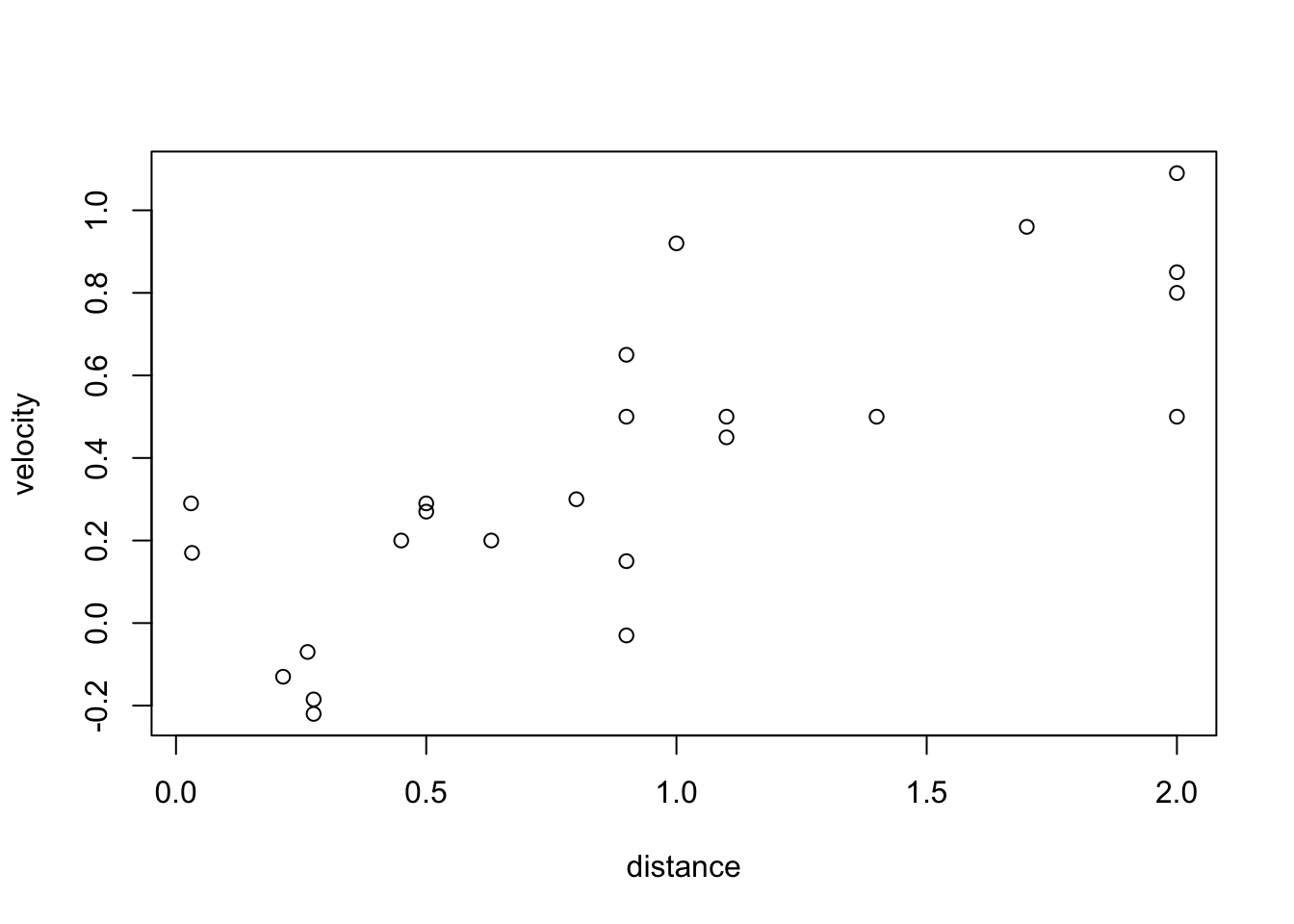

Building a Bayesian regression model

Goal:

designing a model containing a “slope” parameter,
from which we will compute \(\mathbb{E}[\text{slope} | \text{data}]\).

To achieve our goal, we will complete the gap in the following code:

source("../../solutions/simple.R")

regression = function() {
  # priors will be defined here
  # ...
  for (i in 1:nrow(df)) { 
    distance = df[i, "distance"]
    velocity = df[i, "velocity"]
    # likelihood will be defined here
  }
  return(slope)
}

posterior(regression, 1000)

Recall: to build a model, start with the observations.
Specifically, let us build a model for the observed velocity first.

Question: what would be a reasonable likelihood for the velocity?

Question: complete the code and approximate \(\mathbb{E}[\text{slope} | \text{data}]\).

Visualization of the posterior distribution

source("../blocks/simple_utils.R")
source("../../solutions/simple.R")

posterior = posterior_particles(regression, 10000)
weighted_scatter_plot(posterior, plot_options = list(xlab="slope parameter", ylab="sd parameter"))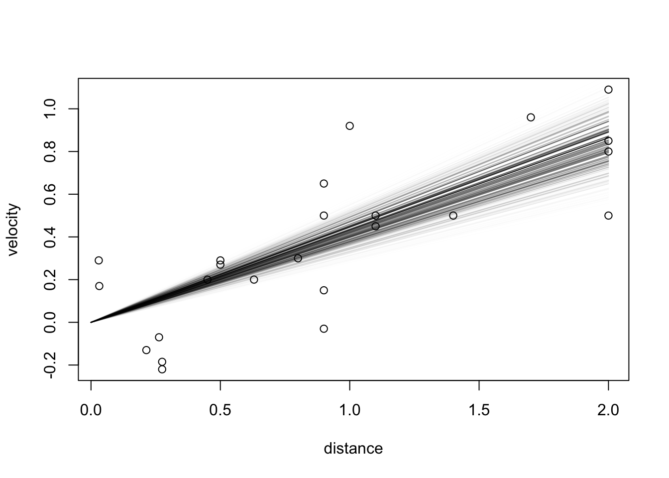

plot(df$distance, df$velocity, xlab = "distance", ylab = "velocity")

xs = seq(0, 2, 0.01)
samples = posterior$samples 
norm_weights = posterior$weights / sum(posterior$weights)

for (i in 1:nrow(samples)) {
  slope     = samples[i, 1]
  pr = norm_weights[i]
  lines(xs, slope * xs, col = rgb(red = 0, green = 0, blue = 0, alpha = pr*20))
}

Here since the scientific question only concerns one parameter, the slope, it is useful to look at the marginal posterior distribution.

In mathematical expressions, obtained by marginalization: \[p(x_1 | y) = \int p(x_1, x_2 | y) \mathrm{d}x_2.\]
In Monte Carlo methods, much simpler:
- each sample is a pair \(x^{(m)}= (x_1^{(m)}, x_2^{(m)})\)
- if you are interested in \(x_1\) only, just ignore \(x_2\)!

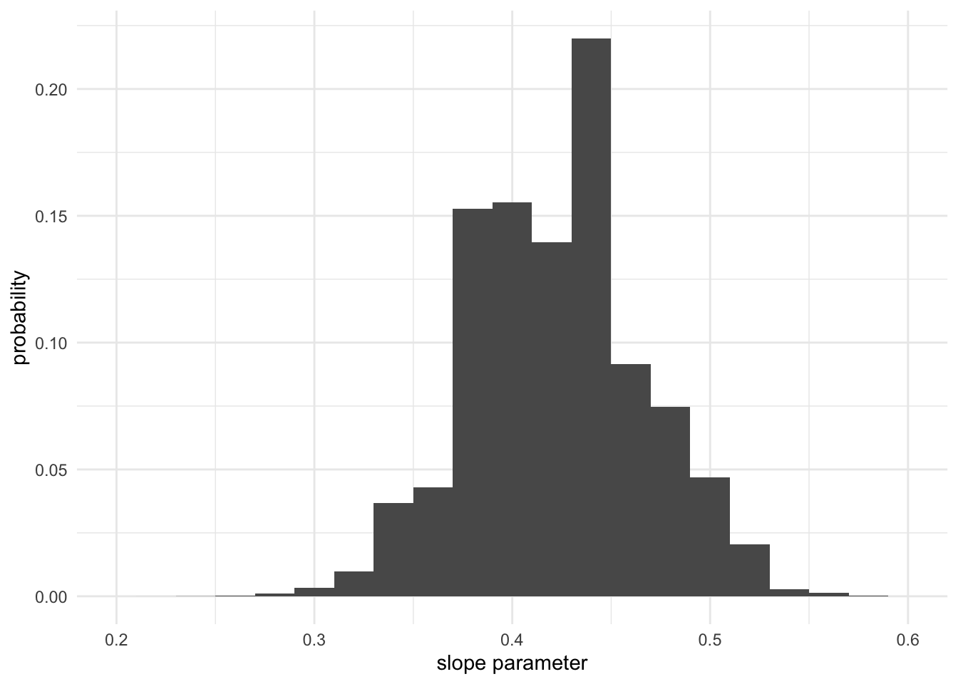
Here is an example of creating a histogram for the marginal posterior:

library("ggplot2")
posterior.as.df <- data.frame(slopes = samples[,1], norm_weights)
ggplot(posterior.as.df, aes(x = slopes, weight = norm_weights)) + 
  geom_histogram(binwidth = 0.02) + 
  xlim(0.2, 0.6) +
  xlab("slope parameter") + 
  ylab("probability") +
  theme_minimal()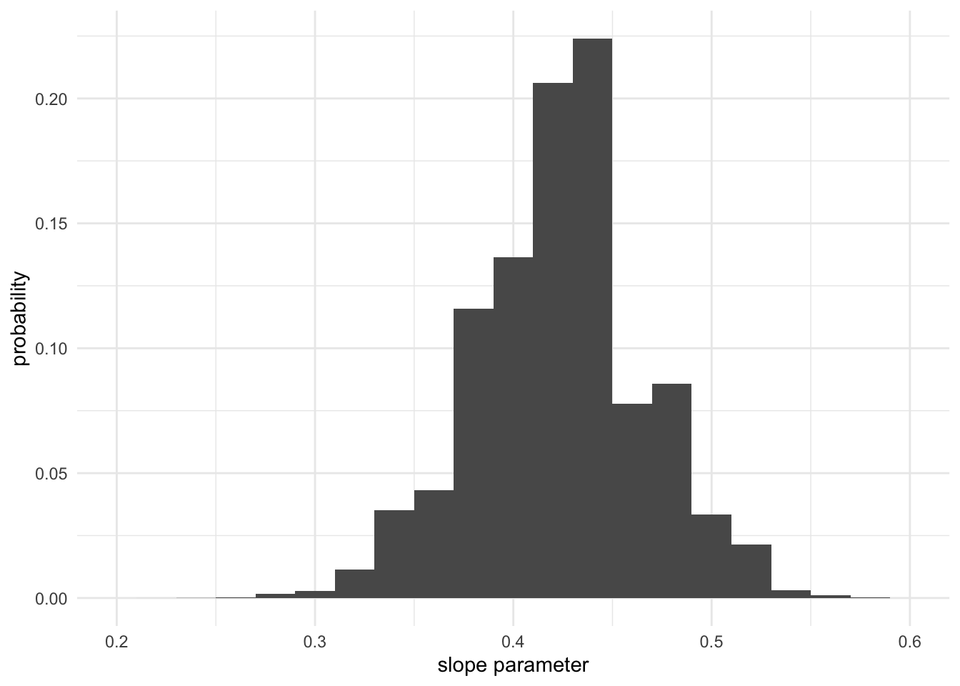

Question: if you were to use an integral instead of Monte Carlo to create this histogram, what region of integration in the scatter plot above (the first plot in this subsection) would be used to compute the height of one histogram bin?

Model criticism

The answer we obtain is close to Edwin Hubble’s original estimate.

The modern estimate based on state-of-the-art measurements (space telescopes, advanced statistical models) gives an estimate that is about 10x smaller.

Discussion: What went wrong?

References

This example is inspired by William Welch’s Stat 305 lecture notes, where the same dataset is analyzed using MLE.
Learn more about the still on-going research on resolving the “Hubble tension”.

Footnotes

Proceedings of the National Academy of Sciences, Vol. 15, pp. 168–173.↩︎