Decision theoretic set estimation
Outline
Topics
- Deriving a set estimate from decision theory.
Rationale
We have seen in week 2 some examples of set estimates (quantile based, highest density set).
These are actually special cases of decision theory with specific choices of loss functions.
This page provides a general framework to answer the question: “how to summarize a posterior distribution with one set?”
Context
- The weakness of point estimates is that they do not capture the uncertainty around the value.
- Idea: instead of returning a single point, return a set of points
- usually an interval,
- but this can be generalized
- Bayesian terminology: credible interval (\(\neq\) frequentist confidence intervals)
- Goals:
- We would like the credible interval to contain a fixed fraction of the posterior mass (e.g. 95%)
- At the same time, we would like this credible interval to be as short as possible given that posterior mass constraint
Bayes estimator formalization
Pick:
- \(A = \{[c, d] : c < d\}\),
- consider the loss function given by \[ L([c, d], x) = \mathbb{1}\{x \notin [c, d]\} + k (d - c) \] for some tuning parameter \(k\) to be determined later.
We get:
\[ \begin{aligned} \delta_{\text{B}}(Y) &= \operatorname{arg\,min}\{ \mathbb{E}[L(a, X) | Y] : a \in A \} \\ &= \operatorname{arg\,min}\{ \Pr[X \notin [c, d] | Y] + k(d - c) : [c,d] \in A \} \\ &= \operatorname{arg\,min}\{ \Pr[X < c|Y] + \Pr[X > d |Y] + k(d - c) : [c,d] \in A \} \\ &= \operatorname{arg\,min}\{ \Pr[X \le c|Y] + 1 - \Pr[X \le d |Y] + k(d - c) : [c,d] \in A \} \\ &= \operatorname{arg\,min}\{ \Pr[X \le c|Y] - \Pr[X \le d |Y] + k(d - c) : [c,d] \in A \} \end{aligned} \]
Here we assume the posterior has a continuous density \(f\) to change \(<\) into \(\le\). We have also used that removing “\(+1\)” does not change the value of the \(\operatorname{arg\,min}\).
As we did with point estimation, we take the derivative with respect to \(c\) and set to zero (then will do the same thing for \(d\)).
Notice that \(\Pr[X \le c|Y]\) is the posterior cumulative distribution function (CDF)1, so taking the derivative with respect to \(c\) yields a density:2
\[ f_{X|Y}(c) - k = 0, \]
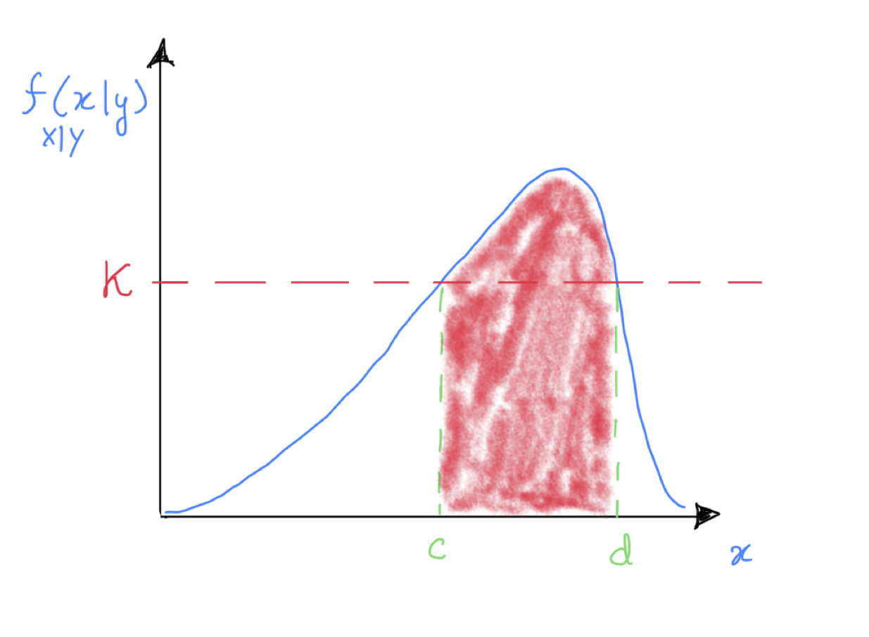
so we see the optimum will be the smallest interval \([c, d]\) such that \(f(c) = f(d) = k\).
Finally, set \(k\) to capture say 95% of the mass (area in red in the figure shows a 50% example, we would lower \(k\) to get to 95%).
Footnotes
Recall that a CDF is defined as \(F(x) = \mathbb{P}(X \le x)\). So a posterior CDF is just \(\mathbb{P}(X \le x | Y)\).↩︎
Let us review the argument why “taking the derivative … yields a density”. Let \(f\) denote a density and \(F\), the CDF of the same random variable. From the definition of a density, \(F(x) = \int_{-\infty}^x f(x') \mathrm{d}x'\) (i.e., take \(A = [-\infty, x]\) in the definition of a density). Hence by the Fundamental theorem of calculus (i.e. the fact that an integral is an “anti-derivative”), we have that \[f(x) = \frac{\mathrm{d}F(x)}{\mathrm{d}x},\] when the derivative exists.↩︎