source("../../solutions/simple.R")
source("../blocks/simple_utils.R")
suppressPackageStartupMessages(library("dplyr"))
set.seed(1)

df = read.csv("../data/launches.csv") %>% filter(LV.Type == "Ariane 1")
success_indicators = df$Suc_bin
rmarkdown::paged_table(df)Bernoulli regression
Outline
Topics
- A first example of a Bayesian model based on a linear model and a Bernoulli likelihood.
- Prior construction via prior predictive distribution.
- Approximation of the posterior using a PPL.
- Visualizing a posterior distribution over functions.
Rationale
- This is our first example of a Bayesian Generalized Linear Model (GLM).
- GLMs are probably some of the most common models.
Example
- The Ariane 1 is an expendable rocket launched 11 times between 1979 and 1986.
- It failed 2 times and was successful the other 9 launches.
- So far our models treat the launches as iid given the success probability \(p\).
- Can we do better?

plot(success_indicators, xlab = "Launch index i")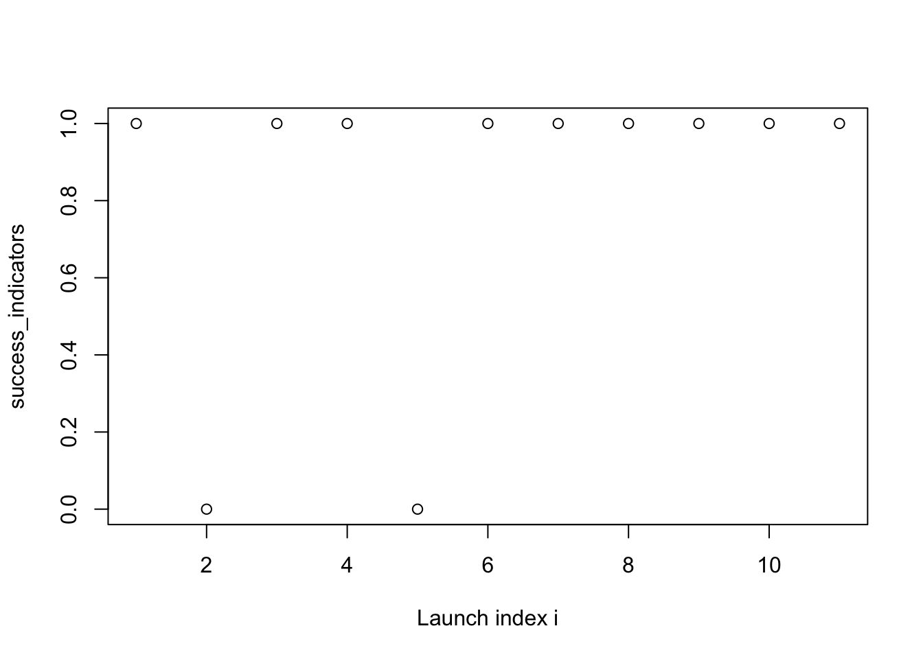
- From this “Exploratory Data Analysis” (EDA), it seems plausible that the success probability is increasing with time.
- Matches with intuition: after a failure, some corrections are made.
Building a better model
- Each observation is binary, so the likelihood still has to be Bernoulli.
- We will denote its parameter by \(\theta \in [0, 1]\).
- What we will change is the prior.
- Old model: \(\theta\) is shared by all launches (“constant over the launch index” \(i \in \{1, 2, \dots, 11\}\))
- New model: \(\theta\) changes from one launch to the next.
- i.e., \(\theta\) is a function of the index \(i \in \{1, 2, \dots, 11\}\), denoted \(\theta(i)\).
- Question: what kind of function should we start with?
- i.e., \(\theta\) is a function of the index \(i \in \{1, 2, \dots, 11\}\), denoted \(\theta(i)\).
CautionClick for answer
General modelling principle: start with something simple!
In our context: start with a linear function.
Structure of the model
- We need to build a prior over linear functions.
- Recall: enough to describe how to forward simulate a dataset.
- Forward simulation process:
- simulate an intercept,
- simulate a slope,
- this determines \(\theta(i)\) for each \(i \in \{1, 2, \dots, 11\}\).
- Simulate \(y_i \sim {\mathrm{Bern}}(\theta(i))\) independently but not identically,
- i.e., we have reduced the problem to that of sampling two real numbers.
- Reasonable prior for a first try: the normal distribution.
Prior (first attempt)
Let us draw one random linear function:
- Math: (not yet final) \[\begin{align*} \text{slope} &\sim \mathcal{N}(0, 1) \\ \text{intercept} &\sim \mathcal{N}(0, 1) \\ \theta(i) &= \text{slope} \cdot i + \text{intercept} \end{align*}\]
- Forward simulation code: (not yet final)
set.seed(1)
plot(success_indicators, ylab = "success probability", xlab = "Launch index i")
xs = 1:length(success_indicators)
intercept = simulate(Norm(0, 1))
slope     = simulate(Norm(0, 1))

lines(intercept + slope * xs)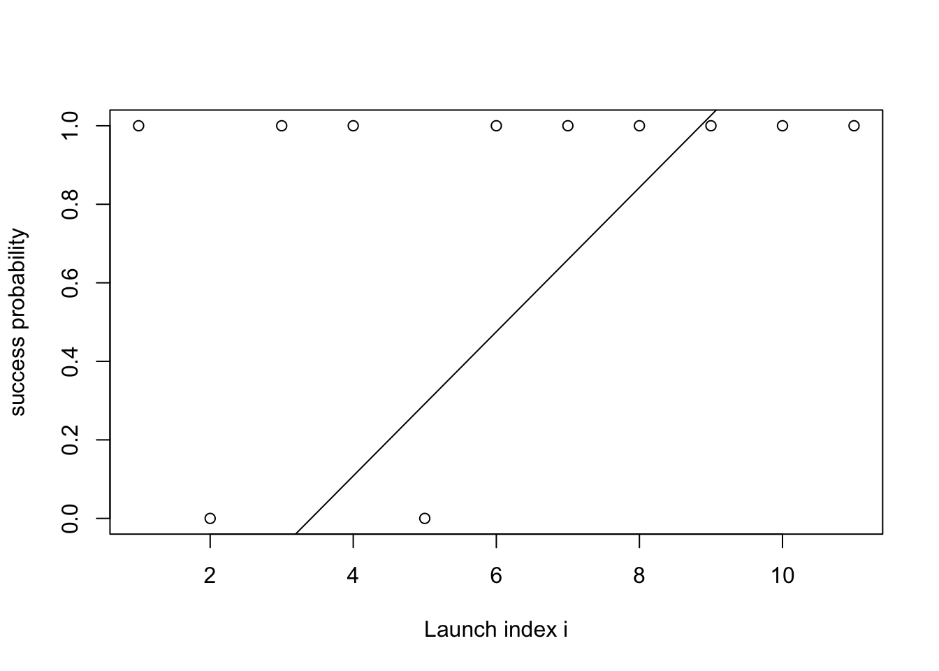
What is the problem in the above?
CautionClick for answer
- The function \(\theta(i)\) can take values smaller than zero or greater than one.
- This creates a problem when we feed the parameter to the Bernoulli, which expects a number between 0 and 1.
Fix:
- we cannot use just a linear function…
- … instead we can compose a linear function with the logistic or sigmoid function.
- Logistic function: maps real numbers \(r \in (-\infty, \infty)\) into \((0, 1)\).
- Math: \[\text{logistic}(r) = \frac{1}{1 + e^{-r}}.\]
- In R:
plogis(r).
rs = seq(-5, 5, 0.01)
plot(rs, plogis(rs), type = 'l', xlab = "r", ylab = "logistic(r)")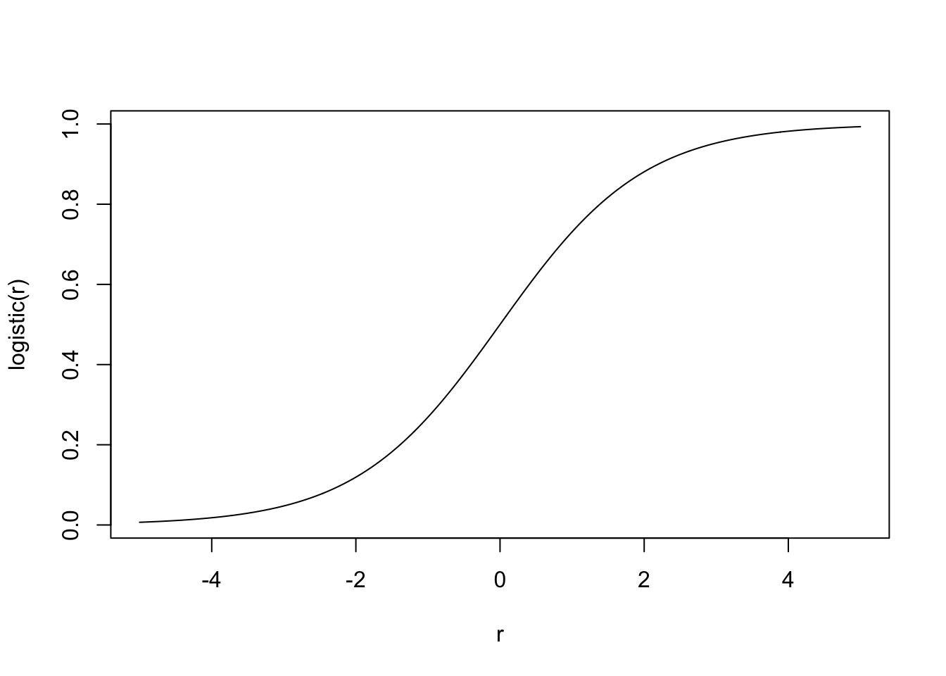
Prior (second, final attempt)
- Math: \[\begin{align*} \text{slope} &\sim \mathcal{N}(0, 1) \\ \text{intercept} &\sim \mathcal{N}(0, 1) \\ \theta(i) &= \text{logistic}(\text{slope} \cdot i + \text{intercept}) \end{align*}\]
- Forward simulation code:
set.seed(1)
plot(success_indicators, ylab = "success probability", xlab = "Launch index i")
xs = 1:length(success_indicators)
intercept = simulate(Norm(0, 1))
slope     = simulate(Norm(0, 1))

lines(plogis(intercept + slope * xs))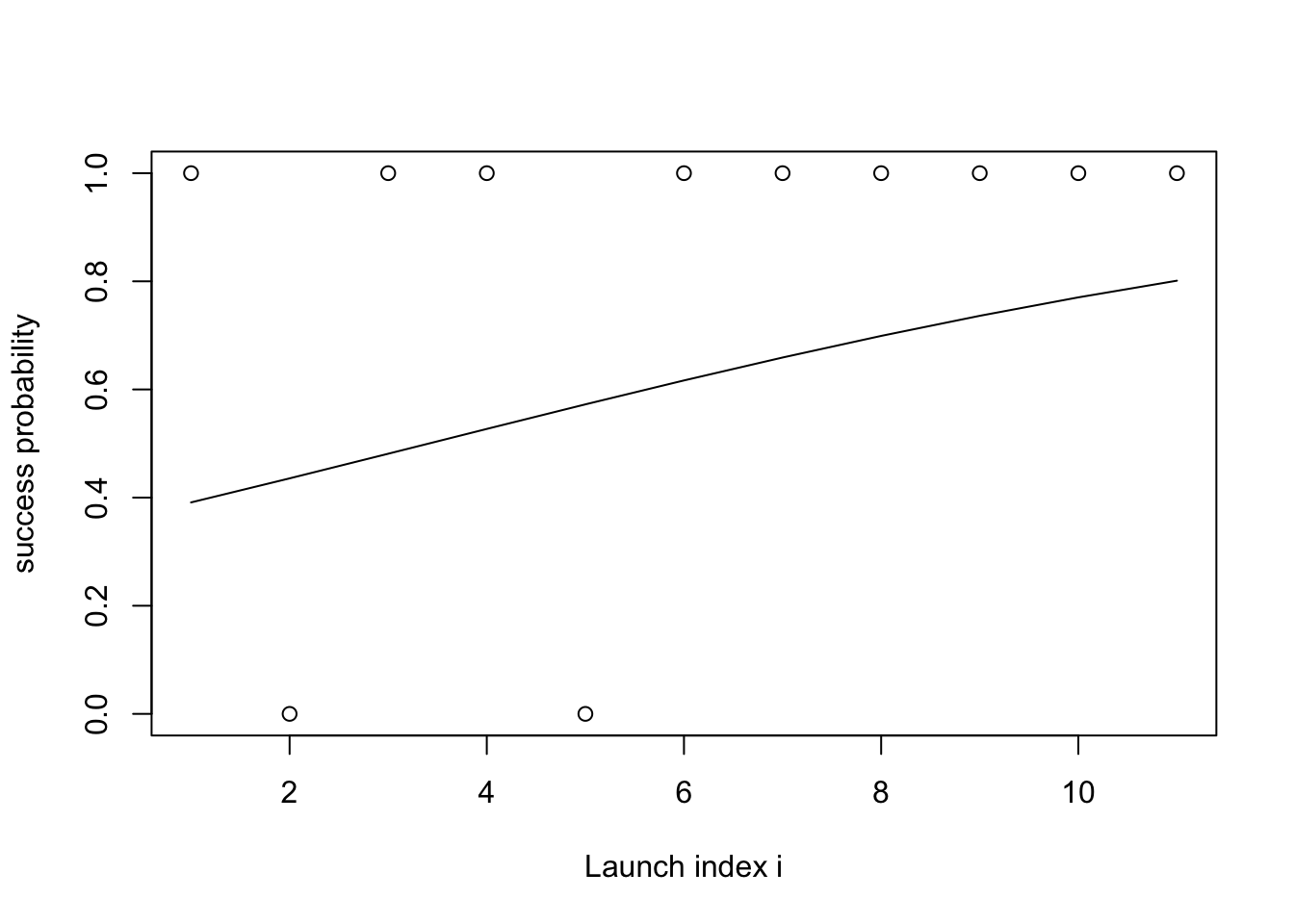
Prior predictive
Let us repeat what we did in the last section 50 times to see several draws from the prior at once (using alpha to make the lines translucent):
set.seed(1)
plot(success_indicators, ylab = "success probability", xlab = "Launch index i")
xs = 1:length(success_indicators)

for (i in 1:50) {
  intercept = simulate(Norm(0, 1))
  slope     = simulate(Norm(0, 1))
  lines(plogis(intercept + slope * xs), col = rgb(red = 0, green = 0, blue = 0, alpha = 0.5))
}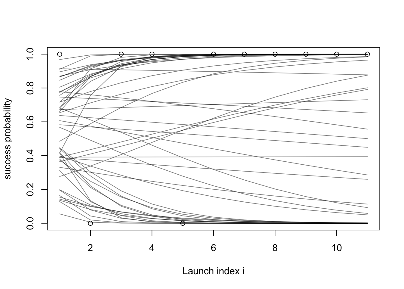
- Hard to get intuition about a prior by just staring at the mathematical formulas.
- Simulating from the prior can help figuring out if the prior is reasonable or not.
- This is known as the prior predictive.
- Exploration:
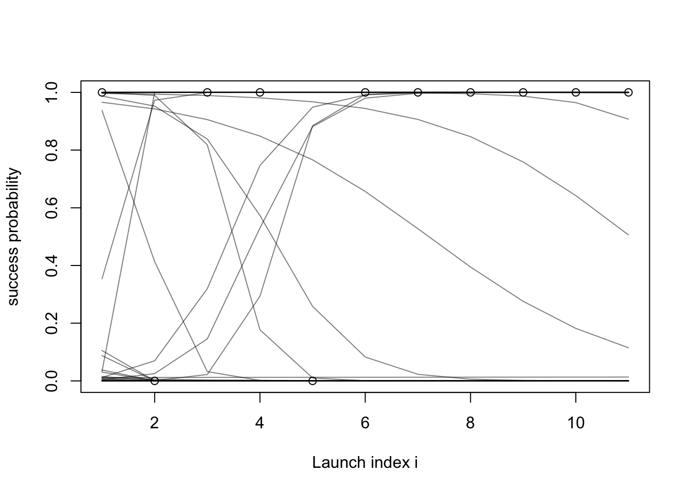
- so far I used a mean of zero and standard deviation of 1 for the slope and intercept priors.
- Let us try a prior that is more “vague”, with standard deviation of 10 for both the slope and intercept priors:
set.seed(1)
plot(success_indicators, ylab = "success probability", xlab = "Launch index i")
xs = 1:length(success_indicators)

for (i in 1:50) {
  intercept = simulate(Norm(0, 10))
  slope     = simulate(Norm(0, 10))
  lines(plogis(intercept + slope * xs), col = rgb(red = 0, green = 0, blue = 0, alpha = 0.5))
}
Posterior distribution
- In this week’s exercise, you will implement the model described above in simPPLe.
- Here is a peek of the posterior distribution you should obtain:
source("../../solutions/sol04_logistic_regression.R")

posterior = posterior_particles(logistic_regression, 1000)
weighted_scatter_plot(posterior, plot_options = list(xlab="intercept parameter", ylab="slope parameter"))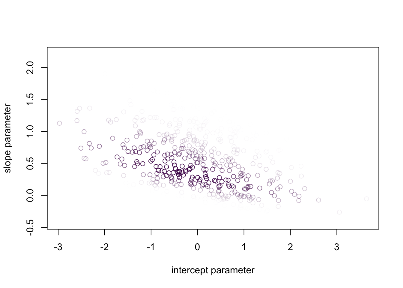
- Again, this is a bit hard to interpret.
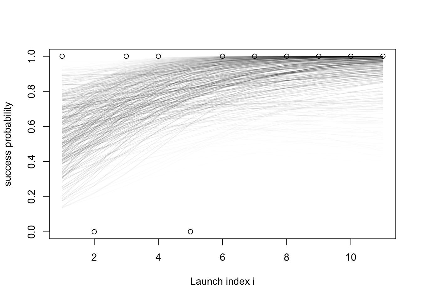
- Let us plot similarly to what we did with the prior predictive:
- For each sample \(x^{(m)}= (\text{intercept}^{(m)}, \text{slope}^{(m)})\) with weight \(w^{(m)}\),
- Draw the curve \(\text{logistic}(\text{slope}^{(m)}\cdot i + \text{intercept}^{(m)})\)…
- with
alphavalue (transparency) proportional to the corresponding weight \(w^{(m)}\).
set.seed(1)
plot(success_indicators, ylab = "success probability", xlab = "Launch index i")
xs = 1:length(success_indicators)

samples = posterior$samples
norm_weights = posterior$weights / sum(posterior$weights)

for (i in 1:nrow(samples)) {
  intercept = samples[i, 1]
  slope     = samples[i, 2]
  pr = norm_weights[i]
  lines(plogis(intercept + slope * xs), col = rgb(red = 0, green = 0, blue = 0, alpha = pr*20))
}
Terminology
The model we just reviewed is an instance of Bayesian logistic regression, a method for classification.
Some terminology from classification:
- output variables: instances of which we try to “predict”
- also known as “target”, “label”, “predicted variable”, “regressand”, …
- sometimes observed (“training instances”), sometimes unobserved (“test instances”)
- in our example?
- input variables: what we use as the basis of each prediction
- also known as “independent variables”, “covariates”, “predictor”, “regressors”, “feature”,..
- typically always observed (both at training and test time)
- parameters: auxiliary quantities that encode a function mapping inputs to (information on) output.