suppressPackageStartupMessages(library(cmdstanr))More Bayesian bricks
Outline
Topics
- More distributions to complement those tested in quiz 1.
- Motivation, realization and parameterization(s) for each.
- Reparameterization.
Rationale
Recall our model building strategy:
- start with observation, and find a distribution that “matches its data type” (this creates the likelihood),
- i.e. such that support of the distribution \(=\) observation data type
- then look at the data types of each of the parameters of the distribution you just picked…
- …and search for a distribution that matches each of the parameters’ data type (this creates the prior),
- in the case of hierarchical models, recurse this process.
There are a few common data types for which we do not have talked much about distributions having realizations of that datatype. We now fill this gap.
Counts
- Support: \(\{0, 1, 2, 3, \dots\}\).

- Simple common choice is the Poisson distribution:
- \({\mathrm{Poisson}}(\lambda)\)
- Parameter: Mean \(\lambda > 0\).
- Motivation: law of rare events.
- Stan doc.
- \({\mathrm{Poisson}}(\lambda)\)
- Popular alternative, e.g., in bio-informatics: the negative binomial distribution:
- \({\mathrm{NegBinom}}(\mu, \phi)\)
- Mean parameter \(\mu > 0\) and concentration \(\phi > 0\).
- Motivation:
- Poisson’s variance is always the same as its mean.
- Consider \({\mathrm{NegBinom}}\) when empirically the variance is greater than the mean (“over-dispersion”).
- Stan doc.
Positive real numbers
- Support: \(\{x \in \mathbb{R}: x > 0\} = \mathbb{R}^+\)

- More common choice is the gamma distribution:
- \({\mathrm{Gam}}(\alpha, \beta)\)
- Parameters: Shape parameter \(\alpha > 0\) and rate \(\beta > 0\).
- Stan doc.
Question: consider the following Stan model:
gamma.stan
data {
  int<lower=0> n_obs;
  vector<lower=0>[n_obs] observations;
}

parameters {
  real<lower=0> shape;
  real<lower=0> rate;
}

model {
  // priors
  shape ~ exponential(1.0/100);
  rate ~ exponential(1.0/100);

  // likelihood
  observations ~ gamma(shape, rate);
}
Notice that neither of the parameters passed in the likelihood can be interpreted as a mean. However, you are asked to report a mean parameter for the population from which the observations come from. How would you proceed?
CautionClick for choices
- Using
generated quantities { real next_obs = gamma_rng(shape, rate); }, and reporting the posterior mean ofnext_obsvariable. - Use the posterior mean of the
shapeparameter, divided by the posterior mean of therateparameter. - Using
transformed parameters { real mean_param = shape/rate; }, and reporting the posterior mean of themean_paramvariable. - All of the above
- None of the above
CautionClick for answer
The most direct is 1, which is in line with what we did for prediction in many examples.
We will see very soon that 3 is also actually possible, this is known as Rao-Blackwellization. In summary, it is based on the fact that if \(Y \sim {\mathrm{Gam}}(\alpha, \beta)\), then \(\mathbb{E}[Y] = \alpha/\beta\).
Empirical example that both are equivalent:
gamma_with_mean.stan
data {
  int<lower=0> n_obs;
  vector<lower=0>[n_obs] observations;
}

parameters {
  real<lower=0> shape;
  real<lower=0> rate;
}

transformed parameters {
  real rao_blackwellized_mean = shape/rate;
}

model {
  // priors
  shape ~ exponential(1.0/100);
  rate ~ exponential(1.0/100);

  // likelihood
  observations ~ gamma(shape, rate);
}

generated quantities {
  real monte_carlo_mean = gamma_rng(shape, rate);
}
set.seed(1)
observations = rgamma(5, shape = 2, rate = 3)
mod = cmdstan_model("gamma_with_mean.stan")
fit = mod$sample(
seed = 1,
refresh = 0,
chains = 1,
data = list(n_obs = length(observations), observations = observations),
iter_sampling = 100000,
output_dir = "stan_out",
)fit$summary(NULL, c("mean"))# A tibble: 5 × 2
variable mean
<chr> <dbl>
1 lp__ -0.661
2 shape 5.92
3 rate 6.64
4 rao_blackwellized_mean 0.922
5 monte_carlo_mean 0.922Counter example that answer 2, a common misconception,1 is incorrect:
5.92 / 6.64[1] 0.8915663This is because we are interested in \(\mathbb{E}[\text{shape}/\text{rate}|Y]\), not \(\mathbb{E}[\text{shape}|Y]/\mathbb{E}[\text{rate}|Y]\).
This can be seen with the (conditional) law of total expectation (reviewed below), and conditional independence of \(Y_\text{next}\) and \(Y_\text{obs}\) given \((\text{shape, rate})\):
\[\begin{align*} \mathbb{E}[Y_\text{next}|Y_\text{obs}] &= \mathbb{E}[ \mathbb{E}[Y_\text{next} | \text{shape, rate}, Y_\text{obs}]|Y_\text{obs}] \\ &= \mathbb{E}[ \text{shape}/\text{rate} |Y_\text{obs}]. \end{align*}\]
An indeed the MC estimates for \(\mathbb{E}[\text{shape}/\text{rate}|Y]\) and \(\mathbb{E}[\text{shape}|Y]/\mathbb{E}[\text{rate}|Y]\) should be expected to be different:
\[ \frac{1}{M} \sum_{m=1}^M \frac{X^{(m)}_\text{shape}}{X^{(m)}_\text{rate}} \neq \frac{\frac{1}{M} \sum_{m=1}^M X^{(m)}_\text{shape}}{ \frac{1}{M} \sum_{m=1}^M X^{(m)}_\text{rate}}. \]
Law of total expectation: \(\mathbb{E}[X] = \mathbb{E}[ \mathbb{E}[X | Y]]\).
Conditional law of total expectation: recall that a conditional probability is a probability. So a good heuristic is that you can take some identity for probabilities and add one random variable to all probability/expectation operators’ conditioning, this yields: \[\mathbb{E}[X | Z] = \mathbb{E}[ \mathbb{E}[X | Y, Z] | Z].\]
Categories
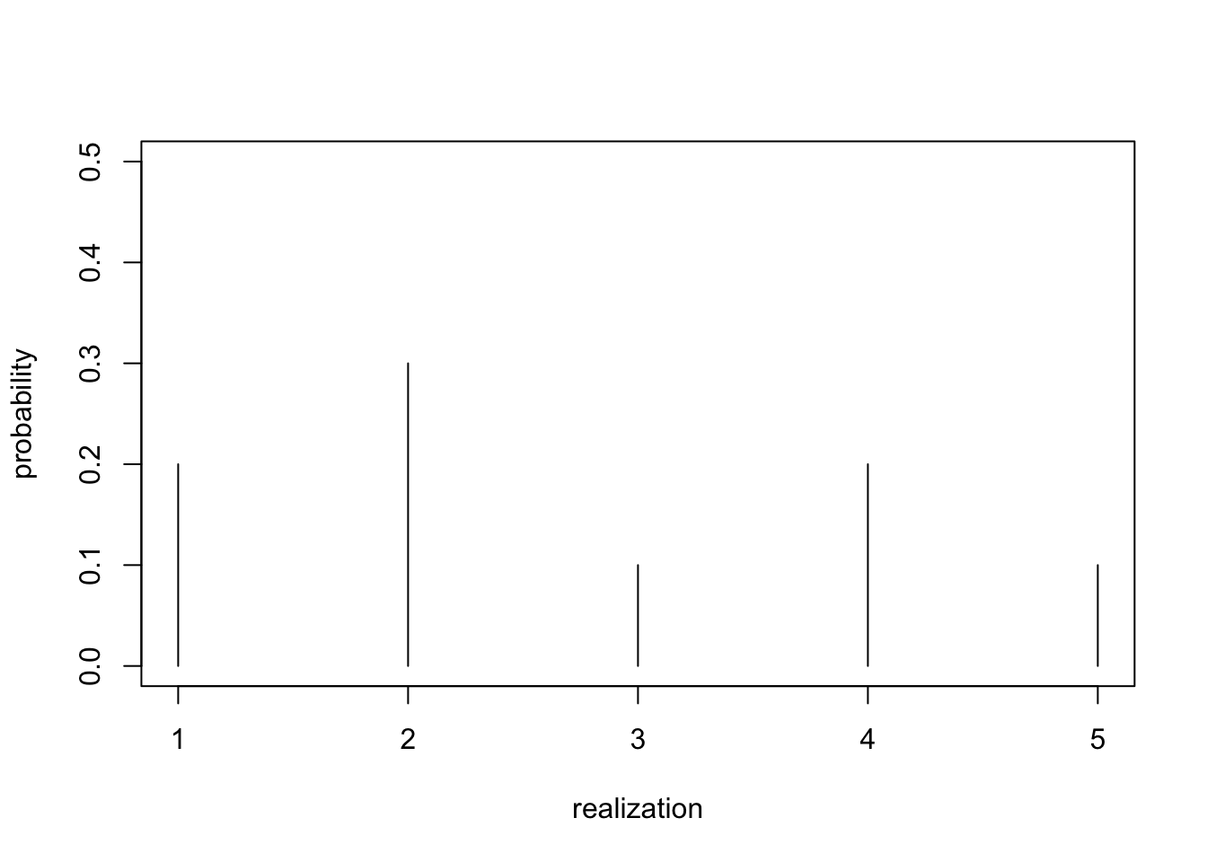
- Support: \(\{1, 2, 3, \dots, K\}\), for some number of categories \(K\).
- All such distributions captured by the categorical distribution
- We first discussed it in Exercise 3.
- \({\mathrm{Categorical}}(p_1, \dots, p_K)\)
- Probabilities \(p_k > 0\), \(\sum_k p_k = 1\).
- Stan doc.
Simplex
Terminology for the set of valid parameters for the categorical, \(\{(p_1, p_2, \dots, p_K) : p_k > 0, \sum_k p_k = 1\}\): the \(K\)-simplex.
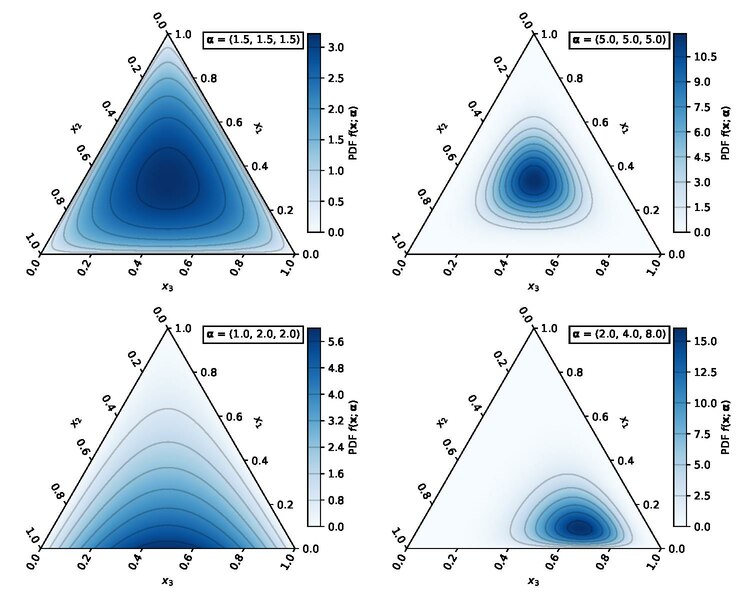
- Hence, if you need a prior over the parameters of a categorical, you need a distribution over the simplex!
- Common choice: the Dirichlet distribution:
- \({\mathrm{Dir}}(\alpha_1, \dots, \alpha_K)\)
- Concentrations \(\alpha_i > 0\).
- Stan doc.
Vectors
- Support: \(\mathbb{R}^K\)
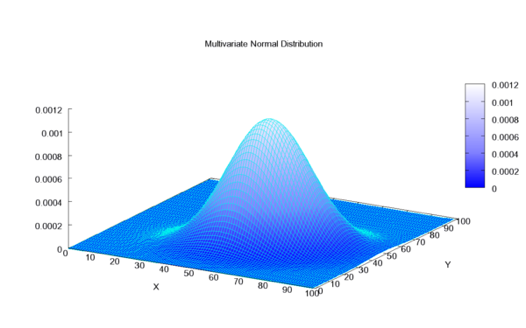
- Common choice: the multivariate normal.
- \(\mathcal{N}(\mu, \Sigma)\)
- Mean vector \(\mu \in \mathbb{R}^K\), covariance matrix \(\Sigma \succ 0\), \(\Sigma\) symmetric.
- Stan doc.
Many others!
References
- Use wikipedia’s massive distribution list,
- and Stan’s documentation.
Alternative approach: reparameterization
- Suppose you need a distribution with support \([0, 1]\).
- We have seen above that one option is to use a beta prior.
- An alternative:
- define \(X \sim \mathcal{N}(0, 1)\),
- use a transformation to map it to \([0, 1]\), e.g. \(Y = \text{logistic}(X)\).
- This approach is known as “re-parametrization”
- For certain variational approaches, this helps inference.
- More on that in the last week.
Footnotes
The root cause of that mis-conception is often an attempt to apply the “plug-in principle” from frequentist statistics to a Bayesian context.↩︎