Data collection mechanisms
Outline
Topics
- Generalizing the censoring problem to other data collection mechanisms.
- Examples of other data collection mechanisms.
Rationale
Rather than memorizing several data collection mechanisms, it is more important to recognize that it is simply a special (but important) example of probabilistic modelling and the first step of our Bayesian recipe.
Truncation
- In censoring, we knew how many \(H_i\)’s were above the detection limit.
- In truncation, a different setup, we now have even less information:
- we only observe the \(H_i\)’s that are below the limit…
- …we don’t know how many were above the limit.
- Mathematically, when the \(H_i\) have a continuous distribution this can be modelled as:
\[\begin{align*} X &\sim \text{prior}() \\ N &\sim \text{DiscreteDistribution}() \\ H_1, \dots, H_N &\sim \text{likelihood}(X) \\ I_i &= \mathbb{1}[H_i \le L] \\ Y &= \{ H_i : I_i = 1 \}. \end{align*}\]
- Here \(I_i\) is an “inclusion indicator”.
- Bayesian analysis will be based on \(X | Y\)
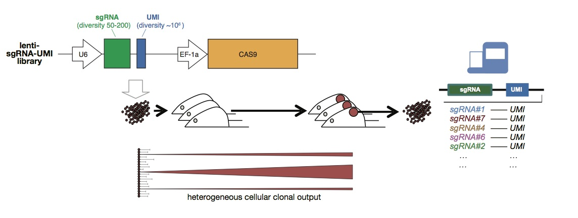
Example: CRISPR-Cas9 unique molecular identifier (UMI) family size. “Families of cells” that left zero progeny are not observed!
Biased data collection
Truncation can be generalized as follows:
- Instead of a deterministic criterion based on \(H_i\) to decide if to include in the set of observations or not,
- make that decision based on some probability model \(p\) that could depend on \(h_i\) and \(x\), \(p(x, h_i) \in [0, 1]\):
\[\begin{align*} X &\sim \text{prior}() \\ N &\sim \text{DiscreteDistribution}() \\ H_1, \dots, H_N &\sim \text{likelihood}(X) \\ I_i &\sim {\mathrm{Bern}}(p(X, H_i)) \\ Y &= \{ H_i : I_i = 1 \}. \end{align*}\]
Question: how would you set \(p(x, h)\) to recover truncation as a special case of biased data collection?
Informative missingness
A related situation is when say you perform a survey by knocking at doors and ask some questions. Some people will refuse to response, and the statistical problem is that the responses for those who refuse to answer might have a different distribution than those who accepted to talk to you and respond to the survey.
Mathematically, this is the same joint distribution as the previous section on biased data collection, but in the survey situation, you get to observe the number of missing values (or equivalently, \(N\) in the mathematical notation used in that section).
Additional readings
See this week’s readings, Chapter 8 of Gelman et al., 2013