Model mis-specification is the norm. What happens to calibration in that case?
Misspecified models and calibration
What to do if your model is misspecified?
One obvious possibility is to make the model better. But in the following we show that under certain conditions, another possibility is to collect more data.
Now suppose we are using the “wrong prior”, i.e.:
data generation uses uniform prior…
…but we base our posterior computation on a different, non-uniform prior.
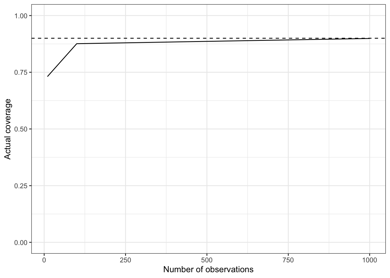
Similarly to the last page, let’s do it for small (10 launches), medium (100), and large datasets (1000), plotting the nominal coverage (dashed) against the actual coverage (solid line)
Code
suppressPackageStartupMessages(library("ggplot2"))suppressPackageStartupMessages(library("dplyr"))suppressPackageStartupMessages(library("tidyr"))theme_set(theme_bw())# Using now the same non-uniform prior as before for posterior calculationK <-1000rdunif <-function(max) { return(ceiling(max*runif(1))) }posterior_distribution <-function(prior_probs, n_successes, n_trials){ K <-length(prior_probs)-1# K+1 values that your p can assume n_fails <- n_trials - n_successes p <-seq(0, 1, 1/K) posterior_probs <-# 1. this computes gamma(i) prior_probs *# - prior p^n_successes * (1-p)^n_fails # - likelihood posterior_probs <- posterior_probs/sum(posterior_probs) # 2. normalize gamma(i) post_prob <-rbind(p, posterior_probs)return(post_prob)}high_density_intervals <-function(alpha, posterior_probs){ ordered_probs = posterior_probs[,order(posterior_probs[2,], decreasing =TRUE)] cumulative_probs =cumsum(ordered_probs[2,]) index =which.max(cumulative_probs >= (1-alpha))return(ordered_probs[,1:index, drop=FALSE])}hdi_coverage_pr <-function(n_datapoints) { n_inclusions <-0for (repetition inseq(1:n_repeats)) { i <-rdunif(K +1) -1# Always generate the data using a uniform prior true_p <- i/K x <-rbinom(1, n_datapoints, true_p) post <-posterior_distribution(prior_used_for_computing_posterior, x, n_datapoints)# This if is just a hacky way to check if true parameter is in the HDI credible intervalif (sum(abs(true_p -high_density_intervals(alpha, post)[1,]) <10e-10) ==1) { n_inclusions <- n_inclusions +1 } }return(n_inclusions/n_repeats) # Fraction of simulation where the true parameter was in interval}prior_used_for_computing_posterior <-dnorm(seq(0, 1, 1/K),mean =0.2, sd=0.2)prior_used_for_computing_posterior <- prior_used_for_computing_posterior /sum(prior_used_for_computing_posterior)set.seed(1)n_repeats <-1000alpha <-0.1df <-data.frame("n_observations"=c(10, 100, 1000))df$coverage_pr <-sapply(df$n_observations, hdi_coverage_pr)ggplot(data=df, aes(x=n_observations, y=coverage_pr)) +ylim(0, 1) +xlab("Number of observations") +ylab("Actual coverage") +geom_hline(yintercept=1-alpha, linetype="dashed", color ="black") +geom_line()
Bad news: for small datasets we are no longer calibrated, in the worst possible way
Higher than the dashed line: would have meant inference is being conservative, i.e. more right than it actually claimed. That’s not too bad.
Lower than the dashed line: we are being overconfident or anti-conservative, which in some cases can be reckless
Good news: in this case, the problem gets quickly corrected as the dataset gets larger. Why?
Asymptotic calibration under misspecification of the prior
There is no general calibration theory for misspecified models, only special cases (outside of that, use simulation studies or cross-validation techniques)
An example where we do have some theory: when the data points \(y_i\) are iid given the parameters \(x\).
Proposition: under certain conditions (outlined below), even when the prior is misspecified, the actual coverage of credible intervals converges to the nominal coverage.
Outline:
the above proposition is a consequence of a stronger result: Bernstein–von Mises theorem (BvM).
BvM theorems provide conditions where the posterior converges to a normal as the data size increases.
Crucially, the parameters of the limiting normal do not depend on the prior!
As a result, when BvM holds, prior misspecification is eventually washed out by the likelihood.
BvM Theorem
Setup:
Assume there is a single true \(x^*\).
Generate datasets of increasing size \(n\),
\(Y_{1:2}, Y_{1:3}, \dots\),
\(Y_{1:n} = (Y_1, \dots, Y_n)\),
\(Y_i \sim p(\cdot | x^*)\).
Consider the sequence of (random) posteriors \(\Pi_n = p(\cdot | Y_{1:n})\)
Result:\(\Pi_n\) approaches a normal distribution.
Which normal distribution?
The same normal that the maximum likelihood estimator converges to!
Centered at \(x^*\),
variance is the inverse of the observed information.