Practice questions

Caution

Page under construction: information on this page may change.

Outline

Topics

• Representative example of questions to prep for Quiz 1.

Important note

The quiz will not focus on multiple choice questions—we use mostly multiple choice in this page just to make it easier to pace the questions during the lecture.

But try to answer before looking at the possible choices to get a more realistic practice!

SNIS

Consider the following partial code for simPPLe’s SNIS engine:

posterior = function(ppl_function, number_of_iterations) {
  numerator = 0.0
  denominator = 0.0
  for (i in 1:number_of_iterations) {
    weight <<- 1.0
    g_i = ppl_function()
    numerator = numerator + weight * g_i
    ???????????????
  }
  return(numerator/denominator)
}

What is the missing line, ????????????????

Click for choices

1. denominator = denominator + g_i
2. denominator = denominator + g_i^2
3. denominator = denominator + weight
4. denominator = denominator + weight^2
5. None of the above.

Click for answer

denominator = denominator + weight

See exercise 3 and the page on simPPLe.

Comparing two parameters

Consider the Bayesian model: for \(i \in \{1, 2\}\),

\[\begin{align*} \theta_i &\sim {\mathrm{Unif}}(0, 1) \\ y_i | \theta_i &\sim {\mathrm{Beta}}(\theta_i). \end{align*}\]

You would like to answer the question: is \(\theta_1\) “clearly different” than \(\theta_2\)? To be concrete, let’s say that “clearly different” means their value differs by at least \(0.1\).

How would you provide a Bayesian answer to the above question?

Click for choices

1. Compute \(\mathbb{P}(|\theta_1 - \theta_2| > 0.1 | y_1, y_2)\).
2. Compute \(\mathbb{E}[\theta_1 | y_1]\) and \(\mathbb{E}[\theta_2 | y_2]\), and check if they differ by more than 0.1.
3. Compute the MAP of \(\theta_1 | y_1\) and of \(\theta_2 | y_2\), and check if they differ by more than 0.1.
4. Compute the posterior median of \(\theta_1 | y_1\) and of \(\theta_2 | y_2\), and check if they differ by more than 0.1.
5. None of the above

Click for answer

Compute \(\mathbb{P}(|\theta_1 - \theta_2| > 0.1 | y_1, y_2)\).

See the page on bivariate posteriors.

Normal distributions

The variability of the normal can be parameterized with the standard derivation, variance, or precision.

Which of the three has the same units of measurement as the mean parameter?

Click for choices

1. Standard deviation.
2. Variance.
3. Precision.
4. None of them.

Click for answer

The standard deviation.

See the page on normal distributions.

Discrete inference

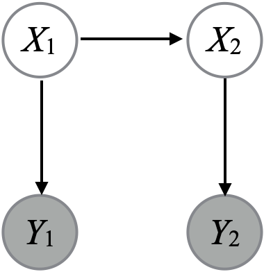
Consider the small HMM on the right defined on binary random variables.

Each edge from a parent random variable to a child in the HMM’s graphical model work the same way: the value of the child is the same as the parent with probability \(2/3\), and it is flipped with probability \(1/3\). The distribution of \(X_1\) is \({\mathrm{Bern}}(1/2)\). Mathematically: \[\begin{align*} X_1 &\sim {\mathrm{Bern}}(1/2) \\ X_2 | X_1 &\sim {\mathrm{Bern}}((2/3)X_1 + (1/3)(1-X_1)) \\ Y_i | X_i &\sim {\mathrm{Bern}}((2/3)X_i + (1/3)(1-X_i)). \end{align*}\]

Compute \(\mathbb{P}(X_2 = 0 | Y_1 = 0, Y_2 = 0)\).

Click for choices

1. \(1/7\)
2. \(2/7\)
3. \(3/7\)
4. \(5/7\)
5. \(8/9\)

Click for answer

Listing the state pairs in the order \((x_1, x_2) \in ((0, 0), (0, 1), (1, 0), (1, 1))\) We have \(\gamma \propto (2^3, 2, 2, 2)\), hence \(\pi = (8/14, 2/14, 2/14, 2/14)\) so \(\mathbb{P}(X_2 = 0 | Y_1 = 0, Y_2 = 0) = 4/7 + 1/7 = 5/7\).

See exercise 1, Bayes rule and detailed derivation of last clicker question in the predictive inference page.

Model construction

Consider the following dataset, showing the monthly number of sun spots from 2010 to 2024:

# source: https://www.sidc.be/SILSO/infosnmtot
suppressPackageStartupMessages(require("dplyr"))
suppressPackageStartupMessages(require("ggplot2"))

df = read.csv("../data/sunspots-SN_m_tot_V2.0.csv", sep = ";", header=FALSE) %>%
        mutate(count = ceiling(V4)) %>%
        rename(year = V3) %>%
        filter(year > 2005)

#by_year = df %>% group_by(year) %>% summarize(count = sum(count))

df %>% ggplot(aes(x = year, y = count)) + geom_point() + ylab("Number of sun spots") + theme_minimal()

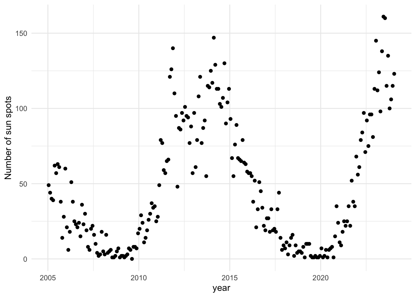
Denote the observations by \(y_i\) where \(i\) is the number of months since January 2005, and \(y_i\) is the number of sun spots observed that month.

Design a Bayesian model to predict the number of sun spots in the next decade. Describe it using the “~” notation. To help you, the following table will be provided during the quiz:

Name	Abbreviation	Parameters
Bernoulli	\({\mathrm{Bern}}(p)\)	Success probability \(p \in [0, 1]\)
Binomial	\({\mathrm{Binom}}(n, p)\)	Number of trials \(n \in \mathbb{N}\), success probability \(p \in [0, 1]\)
Uniform	\({\mathrm{Unif}}(a, b)\)	Left and right bounds, \(a < b\)
Normal	\(\mathcal{N}(\mu, \sigma)\)	Mean \(\mu \in \mathbb{R}\) and standard deviation \(\sigma > 0\)
Exponential	\({\mathrm{Exp}}(\lambda)\)	Rate \(\lambda\) (\(=1/\)mean)
Beta	\({\mathrm{Beta}}(\alpha, \beta)\)	Shape parameters \(\alpha > 0\) and \(\beta > 0\)

Also describe at least one potential source of model mis-specification.

Click for answer

Several possible answers are possible, here is an example:

\[\begin{align*} \theta_1 &\sim {\mathrm{Exp}}(1/1000) \\ \theta_2 &\sim {\mathrm{Exp}}(1/1000) \\ \theta_3 &\sim {\mathrm{Unif}}(0, 2\pi) \\ y_i | \theta &\sim {\mathrm{Poisson}}(\theta_1 (\sin(\theta_2 i + \theta_3) + 1)) \end{align*}\]

Some things we look at:

• The distribution’s support for each variable matches the variable’s datatype.
• The datatype of each distribution parameter is adequate (for example, here \(\theta_1 (\sin(\theta_2 i + \theta_3) + 1) \ge 0\)).
• The model is sufficiently flexible to capture the pattern observed in EDA.

See the page on the step-by-step construction of a GLM.

Many answers possible for model mis-specification. For example, the Poisson distribution will force the mean and variance to be equal, which often does not hold in practice (in this specific example, this might be especially problematic for values \(i\) where \(\sin(\theta_2 i + \theta_3) + 1\) is zero or close to zero).

PPL-based prediction

Recall the model covered in class to perform Bayesian linear regression on galaxy distances and velocities:

regression = function() {
  slope = simulate(Norm(0, 1))
  sd = simulate(Exp(10))
  for (i in 1:nrow(df)) { 
    distance = df[i, "distance"]
    velocity = df[i, "velocity"]
    observe(velocity, Norm(distance * slope, sd))
  }
  c(slope, sd)
}

posterior(regression, 1000)

How would you modify this code to predict the velocity of a galaxy at distance 1.5?

Click for choices

1. Change the line c(slope, sd) to observe(Norm(1.5 * slope, sd))
2. Change the line c(slope, sd) to observe(Norm(1.5, sd))
3. Change the line c(slope, sd) to simulate(Norm(1.5 * slope, sd))
4. Change the line c(slope, sd) to simulate(Norm(1.5, sd))
5. None of the above.

Click for answer

Change the line c(slope, sd) to simulate(Norm(1.5 * slope, sd))

See exercise 4.

Asymptotics

Let \(x\) denote a parameter of interest. The true value is \(x^*\). We have a Bayesian model with \(X\) and \(Y\), and we approximate the posterior mean using SNIS. Let \(\hat G_M\) denote the output of SNIS with test function \(g(x) = x\) and \(M\) iterations.

Where does the following limit converge to? \[\lim_{M\to\infty} \hat G_M = \;?\]

Click for choices

1. \(x^*\)
2. \(\mathbb{E}[X]\)
3. \(\mathbb{E}[X | Y = y]\)
4. \(0\)
5. None of the above.

Click for answer

As discussed in the convergence of SNIS, the correct answer is \(\mathbb{E}[X | Y = y]\).

Beta-binomial conjugacy

Recall that a binomial likelihood has the following PMF: \[p(y | \theta) = \binom{n}{y} \theta^y (1-\theta)^{n-y},\] where \(n\) is the observed number of trials (e.g. launches) and \(y\) is the number of observed successes.

We place a Beta prior on \(\theta\), with hyper-parameters \(\alpha = 1\) and \(\beta = 2\). Recall that beta densities have the following form: \[b_{\alpha, \beta}(\theta) = \frac{1}{Z(\alpha, \beta)} \theta^{\alpha - 1} (1-\theta)^{\beta - 1},\] where \(Z(\alpha, \beta)\) is a normalization constant (i.e. \(Z(\alpha, \beta)\) depends on \(\alpha, \beta\) but not \(\theta\)).

Show that the posterior on \(\theta\) given that we observed 3 successful launches out of 3 (\(y = 3, n = 3\)) has a beta density, i.e., that \[f_{\theta|Y = 3}(\theta) = b_{\alpha', \beta'}(\theta),\] for some \(\alpha', \beta'\).

What is \(\alpha'\) and \(\beta'\)?

Click for choices

1. \(\alpha' = 2, \beta' = 4\)
2. \(\alpha' = 3, \beta' = 0\)
3. \(\alpha' = 3, \beta' = 2\)
4. \(\alpha' = 4, \beta' = 2\)
5. None of the above.

Click for answer

We use the same technique as in Exercise 5, Q1, which is that it is enough to show that \(f_{\theta|Y}(\theta) \propto b_{\alpha', \beta'}(\theta)\) as this will imply they are equal.

By Bayes rule: \[\begin{align*} f_{\theta|Y}(\theta) &\propto b_{\alpha, \beta}(\theta) p(y | \theta) \\ &= \left( \frac{1}{Z(\alpha, \beta)} \theta^{\alpha - 1} (1-\theta)^{\beta - 1} \right) \left(\binom{n}{y} \theta^y (1-\theta)^{n-y}\right) \\ &\propto \theta^{(\alpha + y) - 1} (1-\theta)^{(\beta + n - y) - 1} \\ &= b_{\alpha + y, \beta + n-y}, \end{align*}\] hence \(\alpha' = \alpha + y\) and \(\beta' = \beta + (n-y)\).

In our example here, \(\alpha = 1\), \(\beta = 2\), \(y = 3, n = 3\), so \(\alpha' = 1 + 3 = 4\) and \(\beta' = 2 + (3-3) = 2\).

Credible intervals

You computed two credible intervals based on the same continuous, unimodal posterior distribution: one is a 90% quantile-based interval, the other, a highest density interval (HDI). Which of the intervals is shortest?

Click for choices

1. The quantile-based interval.
2. The HDI interval.
3. It cannot be established with more information.
4. They will always be of equal length.

Click for answer

The HDI interval, by definition.

Decision theory

• A patient is suspected to have a certain disease.
• There is a drastic treatment, which always cures the disease, but costs 1M (in terms of medical facility use and/or physical toll).
• If left uncured, the disease will lead to death which a policy-maker might model as a loss of 10M.

Let \(D\) denote the indicator function on the disease, and \(Y\), data from diagnostic. You posterior gives \(\mathbb{E}[D | Y = y] = 0.2\).

What would a Bayesian recommend?

Click for choices

1. Pick \(a=1\) with probability 0.2.
2. Pick \(a=0\) with probability 0.2.
3. Pick \(a=1\).
4. Pick \(a=0\).
5. Pick either \(a=1\) or \(a=0\) as they incur the same loss.

Click for answer

Let \(a\) denote the indicator that the treatment is used. We get the following losses:

	\(a = 0\)	\(a = 1\)
\(d = 0\)	\(0\)	\(1M\)
\(d = 1\)	\(10M\)	\(1M\)

We compute the expected losses for the two possible actions:

\[\mathbb{E}[L(0, D) | Y = y] = (0.2) (10M) = 2M\]

and

\[\mathbb{E}[L(1, D) | Y = y] = 1M\]

Hence the action that minimizes the loss is \(a = 1\), i.e. to use the treatment.

Posterior expectation

A discrete random variable \(X\) can take values \(-1, 2, 5\). Suppose its posterior PMF given \(Y\) is proportional to: \[\gamma \propto (0.2, 0.1, 0.2).\] Compute \(\mathbb{E}[X^2 | Y]\).

Click for choices

1. 56/5 = 11.2
2. 23/25 = 0.92
3. 19/25 = 0.76
4. 17/25 = 0.68
5. None of the above.

Click for answer

We first compute \(\pi\) by normalization: \[\pi = \frac{\gamma}{0.2 + 0.1 + 0.2} = (2/5, 1/5, 2/5).\]

We can then compute the conditional expectation using LOTUS: \[\mathbb{E}[X^2 | Y] = (-1)^2 (2/5) + 2^2 (1/5) + 5^2 (2/5) = 56/5.\]

See Exercise 1 and expectations review.

Non-standard loss minimization

Derive the Bayes estimator for the loss \(L(a, x) = x^2 - 10ax + a^2\). The posterior mean is \(\mathbb{E}[X | Y = y] = 1\) and \(\operatorname{Var}[X | Y = y] = 1\).

Click for choices

1. 1
2. 5
3. 10
4. 15
5. None of the above

Click for answer

We proceed as in the square loss example:

\[ \begin{aligned} \delta_{\text{B}}(Y) &= \operatorname{arg\,min}\{ \mathbb{E}[L(a, X) | Y] : a \in A \} \\ &= \operatorname{arg\,min}\{ \mathbb{E}[ X^2 - 10aX + a^2 | Y] : a \in A \} \\ &= \operatorname{arg\,min}\{ - 10 a\mathbb{E}[X | Y] + a^2: a \in A \}. \end{aligned} \]

Computing the derivative with respect to \(a\) and setting to zero: \[-10 \mathbb{E}[X | Y] + 2a = 0,\] hence the Bayes estimate or Bayes action is \(a = 10\mathbb{E}[X | Y] / 2 = 5\).

Notation

Which of the following statement(s), if any, follow(s) the notation used in class (i.e., make sense)?

1. \(\mathbb{P}(X) \in [0, 1]\), where \(\mathbb{P}\) is a probability function and \(X\) is a random variable.
2. \(p(x) \in [0, 1]\), where \(p\) is a PMF and \(x\) is a realization.
3. \(\mathbb{P}(x) \in [0, 1]\), where \(\mathbb{P}\) is a PMF, and \(x\) is a realization.
4. \((X = 1) \subset S\), where \(X\) is a random variable and \(S\) is the sample space.
5. \(\mathbb{E}[X + x] = \mathbb{E}[X] + x\), where \(x\) is a realization
6. \(f(x) \in [0, 1]\), where \(f\) is a density.

Click for choices

1. d, e, f
2. a, b, d, e, f
3. a, b, d, e
4. b, d, e
5. None of the above.

Click for answer

Correct choice is: b, d, e

• a, c are incorrect since \(\mathbb{P}\) takes events as input, and \(\mathbb{P}\) is not a PMF but a probability function.
• f is incorrect since a density can be greater than one.

Optimality of Bayes estimator

State the theoretical guarantee that a Bayes estimator \(\delta_{\text{B}}\) has compared to another estimator \(\delta_{\text{o}}\) in terms of average loss.

Click for choices

1. \(\delta_{\text{B}}\le \delta_{\text{o}}\)
2. \(\mathbb{E}[\delta_{\text{B}}] \le \mathbb{E}[\delta_{\text{B}}]\)
3. \(\mathbb{E}[L(\delta_{\text{B}}(Y), X) | Y] \le \mathbb{E}[L(\delta_{\text{o}}(Y), X) | Y]\)
4. \(\mathbb{E}[L(\delta_{\text{B}}(Y), X) | Y] \le 0\)
5. None of the above.

Click for answer

None of the above. The correct inequality is: \[\mathbb{E}[L(\delta_{\text{B}}(Y), X)] \le \mathbb{E}[L(\delta_{\text{o}}(Y), X)].\]

Bias of MC methods

Define formally the notion of bias of a Monte Carlo method.

We have covered two Monte Carlo methods: simple Monte Carlo and SNIS. Which one has the smallest bias?

Click for choices

1. SNIS has smaller bias.
2. Simple Monte Carlo has smaller bias.
3. They cannot be compared in general.
4. Always equal.

Click for answer

The bias is defined as \(\hat G_M - g^*\).

From our discussion on Monte Carlo convergence rate, simple Monte Carlo has a bias of zero, while SNIS is biased.