HMC basics
Outline
Topics
- Intuition
- Conservation of energy
- Augmentation
Intuition
- Let \(\pi\) denote our target density.
- Take the log and take the negative: \(U(x) = - \log \pi(x)\).
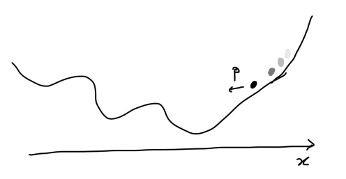
- Now imagine a marble rolling on the landscape \(U(x)\).
- Position at time \(t\): \(x^{(t)} \in \mathbb{R}^d\)
- Momentum at time \(t\): \(p^{(t)} \in \mathbb{R}^d\)
- If you are rusty with physics, for today since we use marbles of mass one, think of momentum = velocity.
- HMC at a high level:
- proposal: from the current position, let the marble roll for time \(t\) (approximately)
- the position at time \(t\) is the proposal.
- Perform an MH accept/reject step based on that proposal.
- Sample a new momentum.
- proposal: from the current position, let the marble roll for time \(t\) (approximately)
Conservation of energy
Why would “rolling a marble on \(U\)” be a good proposal?
Key insight: ignoring friction, recall from elementary physics that we have energy conservation, \[\begin{align*} \text{Hamiltonian}^{(t)} &:= \text{potential energy}^{(t)} + \text{kinetic energy}^{(t)} = \text{constant} \end{align*}\] where: \[\begin{align*} \text{potential energy}^{(t)} &:= U(x^{(t)}), \\ \text{kinetic energy}^{(t)} &:= K(p^{(t)}) := \frac{1}{2} \sum_{i=1}^d (p_i^{(t)})^2, \\ \text{Hamiltonian}^{(t)} &:= H(x^{(t)}, p^{(t)}) = U(x^{(t)}) + K(p^{(t)}). \end{align*}\]
Formalizing this idea:
- Let \(\bar \pi(x, p) \propto \exp(-H(x, p))\).
- Note: the original target \(\pi\) is a marginal of \(\bar \pi\): \[\begin{align*} \int \bar \pi(x, p) \mathrm{d}p &\propto \int \exp(-U(x)) \exp(-K(p)) \mathrm{d}p \\ &= \exp(-U(x)) \int \exp(-K(p)) \mathrm{d}p \\ &\propto \pi(x), \end{align*}\] using that \(\exp(-K(p))\) is proportional to a standard normal density.
- Hence if we can get samples from \(\bar \pi\) we automatically get samples from \(\pi\)!
- Just discard the momenta \(p\).
- Finally:
- if we propose \((x^{(t)}, p^{(t)})\) by “rolling a marble on \(U\)”, starting at the current point \((x^{(0)}, p^{(0)})\)
- we get \(\text{Hamiltonian}^{(t)} = \text{Hamiltonian}^{(0)}\),
- i.e. \(\bar \pi(x^{(t)}, p^{(t)}) = \bar \pi(x^{(0)}, p^{(0)})\),
- i.e. the MH ratio is one, so we automatically accept!
- In practice, we need to approximate the motion of the “rolling marble” so we get \(\bar \pi(x^{(t)}, p^{(t)}) \approx \bar \pi(x^{(0)}, p^{(0)})\) instead.
Augmentation
- The general idea of adding an extra variable to help sampling (like \(p\) here) is frequently used to design MCMC algorithms.
- Terminology:
- the variable we add (e.g. \(p\) here), is called an auxiliary variable,
- the joint distribution over the auxiliary variable and the one of interest \(x\) is called the augmented distribution \(\bar \pi(x, p)\).
- Generally, we want \(\int \bar \pi(x, p) \mathrm{d}p = \pi(x)\) so that we can easily recover the sample of interest.
Sampling a new momentum
- Notice that \(K\) is a quadratic function.
- Hence, \(\exp(\text{quadratic})\) is just a normal distribution!
- How to sample a new momentum?
- Just sample \(p\) from a standard normal…
- … while keeping \(x\) the same.
- This is an example of Gibbs sampling.
- Denote the above kernel by \(K_\text{gibbs}\).
Proposition: \(K_\text{gibbs}\) is \(\bar \pi\)-invariant.
Proof idea: we show a similar result in the discrete case to simplify notation.
- Suppose \(\bar \pi(x) = \pi_1(x_1) \pi_2(x_2)\), \(x = (x_1, x_2)\) as with HMC
- (to map to the above example, think of \(x_1\) as \(x\) and \(x_2\) as \(p\)).
- Define \(K(x' | x) = \mathbb{1}[x_1 = x'_1] \pi_2(x'_2)\).
- Note we have detailed balance: \[\begin{align*} \bar \pi(x) K(x' | x) &= \pi_1(x_1) \pi_2(x_2) \mathbb{1}[x_1 = x'_1] \pi_2(x'_2) \\ &= \pi_1({\color{red} x'_1}) \pi_2(x_2) \mathbb{1}[x_1 = x'_1] \pi_2(x'_2) \;\;\text{(thanks to the indicator)} \\ &= \pi_1(x'_1) \pi_2(x_2) \mathbb{1}[{\color{red} x'_1 = x_1}] \pi_2(x'_2) \\ &= \pi_1(x'_1) {\color{red} \pi_2(x'_2)} \mathbb{1}[x'_1 = x_1] {\color{red} \pi_2(x_2)} \\ &= \bar \pi(x') K(x | x'), \end{align*}\]
- hence global balance holds.
High-level picture
HMC alternates between two kernels:
- a complicated kernel \(K_\text{hmc}\): “rolling the marble”, combined with MH accept-reject which we will explore in more detail
- a simple kernel \(K_\text{gibbs}\): Gibbs sampling on the momentum.