suppressPackageStartupMessages(library(rstan))
suppressPackageStartupMessages(library(ggplot2))
suppressPackageStartupMessages(library(dplyr))

set.seed(1)

df = read.csv(url("https://raw.githubusercontent.com/UBC-Stat-ML/web447/main/data/launches.csv")) %>% filter(LV.Type == "Ariane 1")
success_indicators = df$Suc_bin
rmarkdown::paged_table(df)Stan: hands on
Outline
We revisit the time-varying Ariane 1 rocket failure probability model to practice the Stan syntax introduced this week.

plot(success_indicators, xlab = "Launch index i")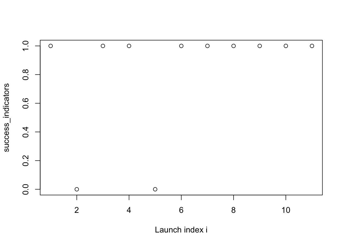
Model
Recall the model we discussed previously (with the difference that we use a SD of 10 now)
\[\begin{align*} \text{slope} &\sim \mathcal{N}(0, 10) \\ \text{intercept} &\sim \mathcal{N}(0, 10) \\ \theta(i) &= \text{logistic}(\text{slope} \cdot i + \text{intercept}) \\ y_i &\sim {\mathrm{Bern}}(\theta(i)) \end{align*}\]
…which you also implemented in simPPLe as part of exercise 4:
logistic_regression = function() {
  intercept = simulate(Norm(0, 10))
  slope     = simulate(Norm(0, 10))
  for (i in seq_along(success_indicators)){
    success_probability = plogis(intercept + i*slope)
    observe(success_indicators[i], Bern(success_probability))
  }
  return(c(intercept, slope))
}
Translation into Stan
Question 1: use the template below to translate the above model into Stan. Set the seed to 1, run 10000 MCMC iterations, and report the posterior mean of the slope parameter.
data {
  int N;
  array[N] int y;
}

parameters {
  real slope;
  real intercept;
}

model {
  // complete this
}
CautionClick for choices
The value closest to the posterior mean of the slope parameter is…
- 0.6
- 0.3
- 0.1
- -0.7
- None of the above
CautionClick for answer
logistic.stan
data {
  int N;
  array[N] int y;
}

parameters {
  real slope;
  real intercept;
}

model {
  slope ~ normal(0, 10);
  intercept ~ normal(0, 10);
  for (i in 1:N) {
    y[i] ~ bernoulli(inv_logit(intercept + slope * i));
  }
}
suppressPackageStartupMessages(library(cmdstanr))
mod <- cmdstan_model("logistic.stan")
fit = mod$sample(
  seed = 1,
  chains = 1,
  refresh = 1000,
  output_dir = "stan_out",
  data = list(
          y = success_indicators,
          N = length(success_indicators)
        ),
  iter_sampling = 10000
)
fit variable mean median sd mad q5 q95 rhat ess_bulk ess_tail
lp__ -5.50 -5.17 1.09 0.79 -7.72 -4.44 1.00 2757 3378
slope 0.56 0.50 0.42 0.39 -0.02 1.33 1.00 2121 2708
intercept -0.65 -0.65 1.80 1.72 -3.69 2.27 1.00 2265 2840Hence the correct choice was 0.6.
Using the posterior
Question 2: compute a 90% credible interval on the slope parameter.
CautionHint
Use the output of print on the fit object.
CautionClick for choices
- \([-4.5, 3.0]\)
- \([0.0, 1.3]\)
- \([-0.1, 1.6]\)
- \([0.3, 1.0]\)
- None of the above
CautionClick for answer
Using again the print out of the fit object:
fit variable mean median sd mad q5 q95 rhat ess_bulk ess_tail
lp__ -5.50 -5.17 1.09 0.79 -7.72 -4.44 1.00 2757 3378
slope 0.56 0.50 0.42 0.39 -0.02 1.33 1.00 2121 2708
intercept -0.65 -0.65 1.80 1.72 -3.69 2.27 1.00 2265 2840We can get a quantile-based credible interval by looking at the columns q5 and q95 (i.e., chopping off 10%/2 on each side): this yields \([-0.02, 1.33]\).
Question 3: translate “your updated belief that the Ariane 1 rockets were improving” into a mathematical expression.
CautionClick for choices
- \(\mathbb{E}[\text{slope}| Y = y] > 0\)
- \(\mathbb{E}[\text{slope}] > 0\)
- \(\mathbb{P}(\text{slope} > 0 | Y = y)\)
- \(\mathbb{P}(\text{slope} > 0)\)
- None of the above
CautionClick for answer
“Ariane 1 rockets were improving” translates to the event \((\text{slope} > 0)\). Hence our “updated belief,” which is just the posterior probability, is \(\mathbb{P}(\text{slope} > 0 | Y = y)\).
Question 4: estimate the numerical value of the expression in the last question.
CautionClick for choices
- 0.65
- 0.75
- 0.85
- 0.94
- None of the above
CautionClick for answer
Here we want to add a new random variable to our model, defined as: \[\text{slope\_is\_positive} = \mathbb{1}[\text{slope} > 0].\] Why? Because then the posterior mean of the indicator will yield the required probability: \[\mathbb{E}[\mathbb{1}[\text{slope} > 0]|Y = y] = \mathbb{P}(\text{slope} > 0 | Y = y),\] and we will be able to read off that mean from the print out of the fit object.
Now, how to add the slope_is_positive random variable to our Stan model?
Since the random variable is defined using “=” rather than “\(\sim\)”, we can do this using a transformed parameters, introduced earlier this week.
Here though notice that is_slope_positive is not used within the model block, in such case, an alternative is to use a generated quantities, which we demonstrate below. Compared to transformed parameters, one advantage of generated quantities is that it is faster (because it only needs to be computed when a sample is collected, for example, if a point is rejected, Stan will skip the computation of the generated quantities for that point, similarly, when the proposal requires intermediate computation as in HMC, generated quantities can be skipped).
logistic_with_generated.stan
data {
  int N;
  array[N] int y;
}

parameters {
  real slope;
  real intercept;
}

model {
  slope ~ normal(0, 10);
  intercept ~ normal(0, 10);
  for (i in 1:N) {
    y[i] ~ bernoulli(inv_logit(intercept + slope * i));
  }
}

generated quantities {
  real is_slope_positive = slope > 0 ? 1 : 0;
}
suppressPackageStartupMessages(library(cmdstanr))
mod <- cmdstan_model("logistic_with_generated.stan")
fit = mod$sample(
  seed = 1,
  chains = 1,
  refresh = 1000,
  output_dir = "stan_out",
  data = list(
          y = success_indicators,
          N = length(success_indicators)
        ),
  iter_sampling = 10000
)fitWarning: NAs introduced by coercion variable mean median sd mad q5 q95 rhat ess_bulk ess_tail
lp__ -5.50 -5.17 1.09 0.79 -7.72 -4.44 1.00 2757 3378
slope 0.56 0.50 0.42 0.39 -0.02 1.33 1.00 2121 2708
intercept -0.65 -0.65 1.80 1.72 -3.69 2.27 1.00 2265 2840
is_slope_positive 0.94 1.00 0.24 0.00 0.00 1.00 1.00 2935 NAHence the correct answer is 0.94, the posterior mean of is_slope_positive.