Bivariate posteriors

Outline

Topics

  • Posterior distribution on two parameters (bivariate).

Rationale

There is typically more than one unknown variables. Going from one unknown to two unknowns is the biggest leap.

Example

We will revisit the rocket comparison problem from the first week:

  • Would you rather get strapped to…
    • “shiny rocket” (option A): 1 success, 0 failures
    • “rugged rocket” (option B): 98 successes, 2 failures

  • If you are sick of hearing about rockets, here is an alternative interpretation:
    • Imagine you work for Google and serve website ad banners.
    • A client gives you two designs for the ad banner: A and B.
    • You will serve them to web visitors and the objective is to maximize the number of clicks.
      • Success: a user clicked (1).
      • Failure: a user did not click (0).
    • Training data:
      • Version A: 1 success, 0 failures.
      • Version B: 98 successes, 2 failures
    • You can only show the ad one more time to a user (client budget almost exhausted).
      • Should you show A or B?
    • This is a basic example of what is known as A/B testing.

Model: for \(j \in \{A, B\}\), independently,

\[\begin{align*} p_j &\sim {\mathrm{Unif}}(0, 1) \\ y_j | p_j &\sim {\mathrm{Binom}}(n_j, p_j), \end{align*}\]

where:

  • \(p_j\) are the success probabilities
  • \(n_j\) is the number of times you showed \(j\)
  • \(y_j\) is the number of clicks on \(j\).

Question:

How to mathematically encode the questions:

  • “Would you rather get strapped to…”
  • “Should you show A or B?”
  1. \(\mathbb{P}(p_A = 1)\)
  2. \(\mathbb{P}(p_A = 1 | Y = y)\)
  3. \(\mathbb{P}(p_A > p_B)\)
  4. \(\mathbb{P}(p_A > p_B | Y = y)\)
  5. None of the above

\(\mathbb{P}(p_A > p_B | Y = y)\): in words, is the chance of success of A greater than B, given the data?

Modify the code below to approximate that probability.

source("../../solutions/simple.R")
set.seed(1)

bivariate = function() {
  
  p_A = simulate(Beta(1, 1))
  observe(1, Binom(size = 1, prob = p_A)) 
  
  # add the part of the model describing p_B (prior and likelihood)
  
  return # what is the "test function"?
}
posterior(bivariate, 10000)
  1. \(\approx 0.1\)
  2. \(\approx 0.3\)
  3. \(\approx 0.6\)
  4. \(\approx 0.9\)
source("../../solutions/simple.R")
set.seed(1)

bivariate = function() {
  
  p_A = simulate(Beta(1, 1))
  observe(1, Binom(size = 1, prob = p_A)) 
  
  p_B = simulate(Beta(1, 1))
  observe(98, Binom(size = 100, prob = p_B)) 
  
  return(ifelse(p_A > p_B, 1, 0))
}
posterior(bivariate, 10000)
[1] 0.06909026

Visualization of a bivariate joint posterior

Let us get more insight on joint posterior distributions (posterior over two variables).

To do so, we use visualizations where the x-axis is the first parameter (here \(p_A\)) and the y-axis is the second parameter (here \(p_B\)).

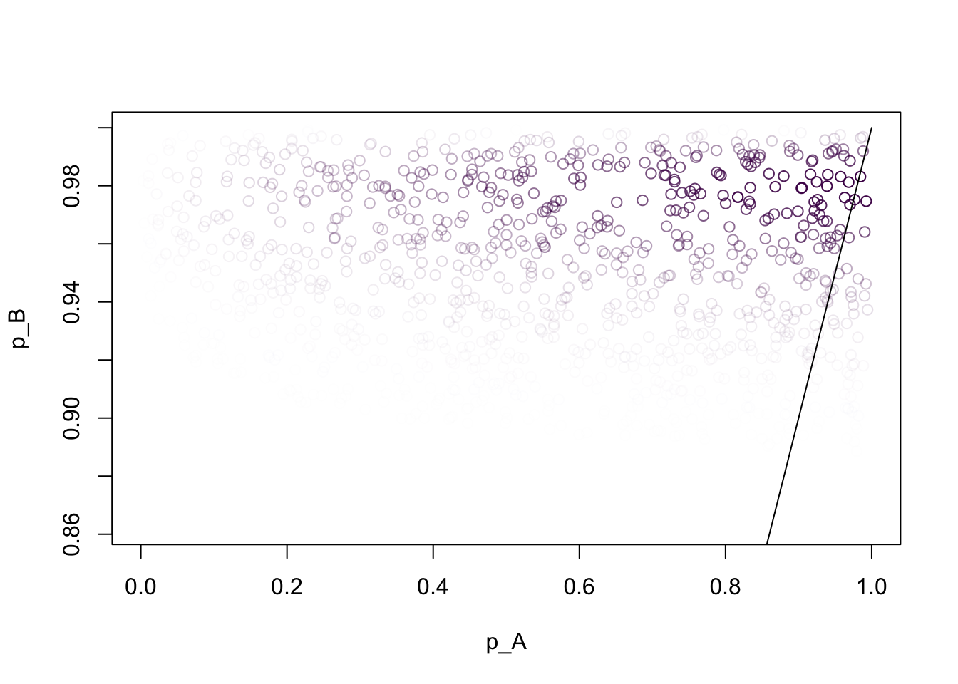
# This contains useful functions to visualize the output of simPPLe:
source("../blocks/simple_utils.R")

bivariate_pair = function() {
  
  p_A = simulate(Beta(1, 1))
  observe(1, Binom(size = 1, prob = p_A)) 
  
  p_B = simulate(Beta(1, 1))
  observe(98, Binom(size = 100, prob = p_B)) 
  
  # We modify the above to return a vector containing both parameters
  c(p_A, p_B)
}

# To compute the plot, we need the list of samples and weights ("particles"), i.e. more details compared to posterior()
# This is what posterior_particles accomplishes
particles = posterior_particles(bivariate_pair, 10000)

# Now we use these to create the plot below
weighted_scatter_plot(particles, plot_options = list(xlab="p_A", ylab="p_B"))

xaxis = seq(0, 1, 0.01)
lines(xaxis, xaxis)

  • Each point is a sample produced by SNIS, \(x^{(m)}= (p_A^{(m)}, p_B^{(m)})\).
  • We encode its associated weight \(w^{(m)}\) by the transparency (alpha) of the point.

Question: What region of integration should you use to compute \(\mathbb{P}(p_A > p_B | Y = y)\)?