Monte Carlo convergence rate

Outline

Topics

• Convergence rate of Monte Carlo methods.
• Empirical scaling laws using physicist’s log-log plot trick.
• Mathematical underpinnings.

Rationale

When using Monte Carlo methods, you need to specify the number of iterations (also known as number of samples).

How to set the number of iterations?

We cover here a heuristic, forming the foundation for more principled methods.

Setup

Important: we go back to simple Monte Carlo here, to make the argument simpler. However our findings will apply equally to SNIS (and later, to MCMC).

Motivating example

Let us revisit Q.1.3 in the first exercise. We will use it to explore tricks to set the number of Monte Carlo iterations.

Setup: coin bag with a single flip (where we write \(Y = Y_1\))

\[ \begin{align*} X &\sim {\mathrm{Unif}}\{0, 1, 2\} \\ Y | X &\sim {\mathrm{Bern}}(X/2) \end{align*} \tag{1}\]

Plan: We will use our forward simulator and the law of large numbers to approximate \(\mathbb{E}[(1 + Y)^X]\).

Recall from the exercise 1 solutions (simplified a bit here):

truth = 1/3 * (1 + 1/2 + 1 + 4)
truth

[1] 2.166667

set.seed(1)
suppressMessages(require(extraDistr))

forward_sample = function() {
  x = rdunif(1, min=0, max=2)
  y = rbern(1, x/2)
  return(c(x, y))
}

simple_monte_carlo = function(n_iterations) {
  sum = 0.0
  for (iteration in 1:n_iterations) {
    sample = forward_sample()
    sum = sum + (1+sample[2])^sample[1]
  }
  return(sum/n_iterations)
}

Let’s run the simulator with 10 iterations:

simple_monte_carlo(10)

[1] 2.3

Is this reliable? Let’s run it two more times:

simple_monte_carlo(10)

[1] 2.7

simple_monte_carlo(10)

[1] 2.1

• OK.. the first digit seems “stabilized” but not the second digit.
• Suppose I want one more digit of accuracy…

By how much should I increase the number of iteration to get one more digit of accuracy?

Click for choices

1. 10 times more iterations
2. 100 times more iterations
3. 1000 times more iterations
4. there is no way to answer this questions
5. None of the above

Empirical scaling

Continuing on the same example (where we know the truth!), we will now:

• vary the number of iterations (\(10^1, 10^{1.5}, 10^2, 10^{2.5}, 10^3\)),
  • for each number of iteration n_iterations, we run simple_monte_carlo(n_iterations) 500 times,
  • and plot the errors in log-log scale.

First, a function to compute the approximation error of one call to simple_monte_carlo(n_iterations):

approximate_error = function(n_iterations) {
  mc = simple_monte_carlo(n_iterations)
  error = abs(mc - truth)
  return(error)
}

Second, running approximate_error on the different numbers of iterations, each 500 times:

df <- data.frame("n_iterations" = rep(c(10, 32, 100, 316, 1000), each=500))
df$errors <- sapply(df$n_iterations, approximate_error)

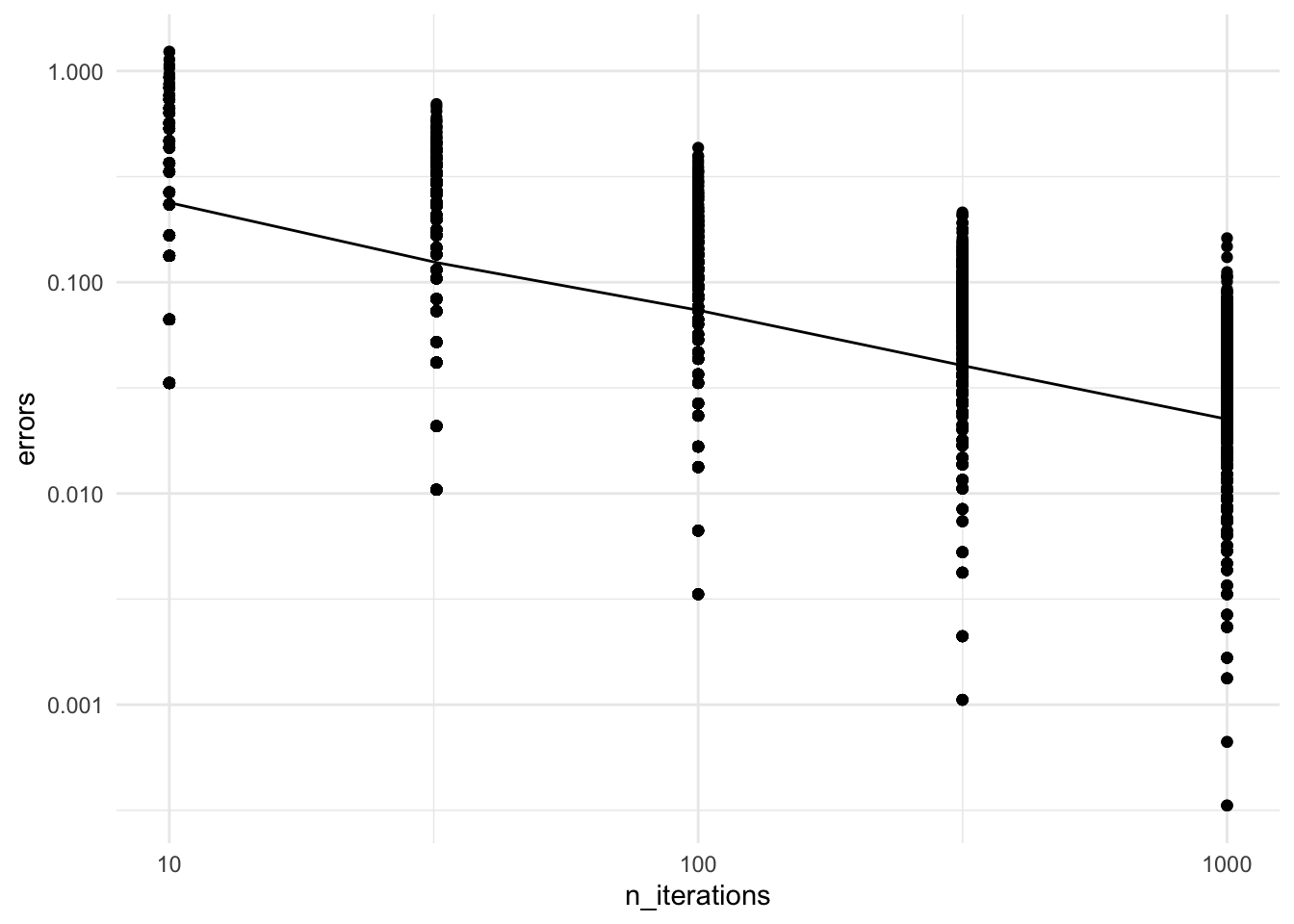
Finally, plotting the errors in log-log scale (each of the \(500 \cdot 5\) points is the error of one Monte Carlo run):

require(ggplot2)

Loading required package: ggplot2

ggplot(data=df, aes(x=n_iterations, y=errors)) +
  stat_summary(fun = mean, geom="line") + # Line averages over 1000 replicates
  scale_x_log10() +  # Show result in log-log scale
  scale_y_log10() +
  theme_minimal() +
  geom_point()

• Good news: error goes to zero

  • Recall this property is known as consistency.
  • This confirms the theory covered on the previous page.
  • But here we are interested in the rate (how fast does it go to zero?)

• Result suggests a linear fit in the log-log scale \(\underbrace{\log_{10}(\text{error})}_{y} = a\; \underbrace{\log_{10}(\text{number of iterations})}_{x} + b\)

• Questions:

  • Eyeball the coefficient \(a = \Delta x / \Delta y\).
  • What can you this coefficient tell you about the scaling of the error?

Click for choices

1. \(2\)
2. \(1/2\)
3. \(1\)
4. \(-1/2\)
5. \(-2\)

Click for answer

• Get \(a \approx -1/2\)

• Hence taking power on each side of

\(\underbrace{\log_{10}(\text{error})}_{y} = a \underbrace{\log_{10}(\text{number of iterations})}_{x} + b\)

• we get that the error will scale like \[\frac{\text{constant}}{\sqrt{\text{number of iterations}}}\]

Based on this extra information, let’s try revisit our initial question: By how much should I increase the number of iteration to get one more digit of accuracy?

Click for choices

1. 10 times more iterations
2. 100 times more iterations
3. 1000 times more iterations
4. there is no way to answer this questions
5. None of the above

Click for answer

• since we now know that the error will scale like \[\frac{\text{constant}}{\sqrt{\text{number of iterations}}}\]

• … if we want to reduce it by factor 10 (i.e. “gain one significant digit”), we need 100x more iterations

• To gain 2 more significant digits: need 10,000x more iterations, etc

• What we did here is an example of an (empirical) asymptotic analysis.

Mathematical underpinnings

Notation: recall \(\hat G_M\) is the estimator. Let us denote the truth by \(g^* = \mathbb{E}[g(X, Y)]\).

Core of the argument: use that for independent random variables \(V_1, V_2\), \(\operatorname{Var}[V_1 + V_2] = \operatorname{Var}[V_1] + \operatorname{Var}[V_2]\)! This gives us:

\[\operatorname{SD}(\hat G_M) = \sqrt{\operatorname{Var}\frac{1}{M} \sum_{i=1}^M G^{(m)}} = \sqrt{\frac{M \operatorname{Var}G^{(1)}}{M^2}} = \frac{\text{constant}}{\sqrt{M}}\]

In the following, I will explain why analyzing the standard deviation makes sense…

Surrogate error measure: Mathematically analyzing the error as we define in our code, \(\mathbb{E}|\hat G_M - g^*|\), is tricky; it is easier to look instead at the Root Mean Squared Error (RMSE): \[\operatorname{RMSE}= \sqrt{\operatorname{MSE}} = \sqrt{ \mathbb{E}[ (\hat G_M - g^*)^2 ]}.\] Sanity check: Note that the units are OK, i.e. the error measured in RMSE and with the more intuitive \(\mathbb{E}|\hat G_M - g^*|\) has the same units, e.g. meters, or grams or whatever, as the estimator \(\hat G_M\) and truth \(g^*\).

It’s enough to study the standard deviation:

• Recall that the MSE is the sum of variance and bias squared (see wikipedia for proof) \[\begin{align*} \operatorname{MSE}&= \operatorname{Var}[\hat G_M] + (\operatorname{Bias}(\hat G_M, g^*))^2 \\ \operatorname{Bias}(\hat G_M, g^*) &= \mathbb{E}[\hat G_M] - g^*. \end{align*}\]
• For simple Monte Carlo, the bias is zero by linearity of expectation:¹ \[\mathbb{E}[\hat G_M] = \mathbb{E}\left[\frac{1}{M} \sum_{m=1}^M G^{(m)}\right] = \frac{1}{M} \sum_{m=1}^M \mathbb{E}[G^{(m)}] = \mathbb{E}[G^{(m)}] = g^*.\]

• The bias of zero gives a simpler expression for RMSE: \[\operatorname{RMSE}= \sqrt{\operatorname{Var}[\hat G_M] + 0} = \operatorname{SD}[\hat G_M]\]
• Hence for simple Monte Carlo, analyzing the scaling of the standard deviation (SD) is the same as analyzing the RMSE.

Contextualizing the error rate of Monte Carlo

• Numerical methods such as the trapezoidal rule converge much faster in terms of \(M\): \[\text{error} = \frac{\text{constant}}{M^2},\] i.e. 10 times more iterations gives two digits of extra accuracy (here \(M\) is the number of grid points used in a 1d numerical integral)!
• So why do we use Monte Carlo?
  • The constants in the analysis of numerical integration blow up exponentially in the dimensionality of the problem!
  • Many Monte Carlo methods can avoid this exponential blow up in the dimensionality.²
  • And good scalability in the dimensionality of the problem often more important than scalability in number of digits of accuracy
    • …can’t trust 10th digit anyways because the model almost always has some amount of mis-specification.

Footnotes

1. For SNIS, the bias is not zero (because we have a ratio), but the squared bias decays faster than the variance term as \(M \to \infty\) so the argument is essentially the same as simple Monte Carlo.

2. In particular, Simple Monte Carlo and MCMC can often avoid the curse of dimensionality. But not SNIS! Why are we spending time on SNIS then? Because it can be used to approximate arbitrary posterior distribution, while simple Monte Carlo cannot, and it is much simpler than MCMC, so a good starting point pedagogically. However we will jump to MCMC later in this course.