Prediction

Outline

Topics

• Prediction using decision trees
• Example

Rationale

Often we do not care so much about “parameters” but instead about predicting future observations.

Example: coins in a bag

Consider the setup from last week with 3 coins and 3 flips with $Y=(1,1,1)$ (in the following, let $\mathbf{1}$ denote a vector of 1’s).

Question: given you have see 3 heads, what is the probability that the next one is also heads?

Mathematically: $\mathbb{P}(Y_4=1|Y_{1:3}=\mathbf{1})$. This is known as “prediction”.

General approach

Key message: In Bayesian statistics, prediction and parameter estimation are treated in the exact same way!

Idea: Add $Y_4$ to the unobserved random variables, i.e. set $\tilde{X}=(X,Y_4)$.

Then, to compute $\mathbb{P}(Y_4=1|Y_{1:3}=\mathbf{1})$ use same techniques as last week (decision tree, chain rule, axioms of probability).

Example, continued

Use the following picture to help you computing $\mathbb{P}(Y_4=1|Y_{1:3}=\mathbf{1})$.

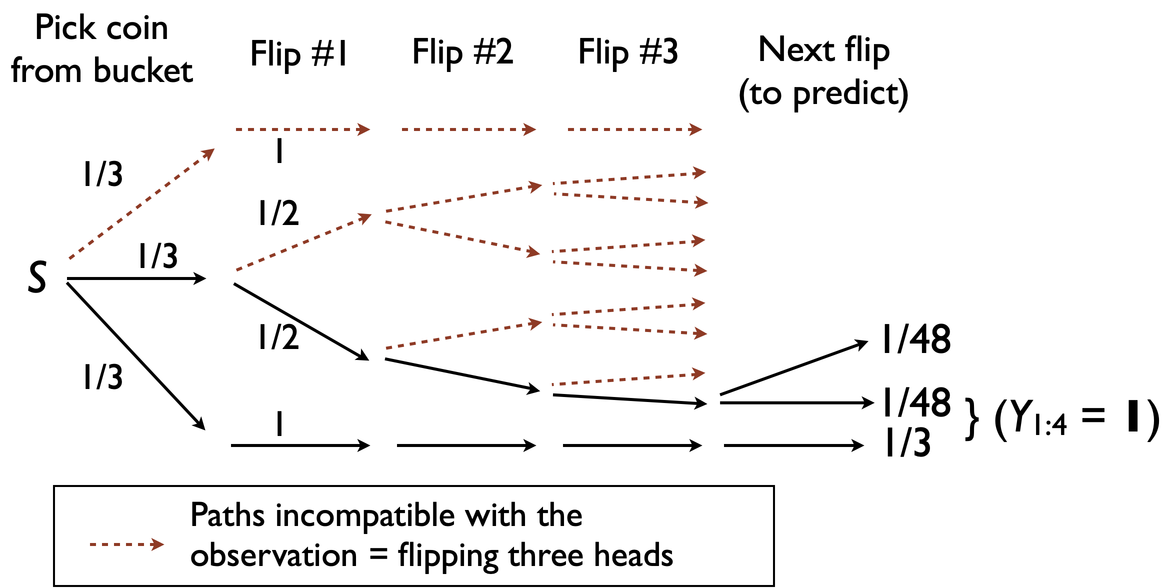
Notation: let $\gamma (i)=\mathbb{P}(Y_{1:3}=\mathbf{1},Y_4=i)$.

Question: compute $\gamma (0)$.

Click for choices

1. $\approx 0.02$
2. $\approx 0.06$
3. $\approx 0.52$
4. $\approx 0.94$
5. None of the above

Click for answer

• There is only one way to get $(Y_{1:3}=\mathbf{1},Y_4=0)$: this has to be the standard coin, i.e., $$(Y_{1:3}=\mathbf{1},Y_4=0)=(X=1,Y_{1:3}=\mathbf{1},Y_4=0)$$
• To compute the probability of that path we can multiply the edge probabilities (why?): $$\gamma (0)=\mathbb{P}(X=1,Y_{1:3}=\mathbf{1},Y_4=0)=(1/3)\times (1/2{)}^4=1/48\approx 0.02.$$

Question: compute $\gamma (1)$.

Click for choices

1. $\approx 0.11$
2. $\approx 0.35$
3. $\approx 0.52$
4. $\approx 0.94$
5. None of the above

Click for answer

• Twist: two distinct paths are compatible with the event: $$(Y_{1:4}=\mathbf{1})=(X=2,Y_{1:4}=\mathbf{1})\cup (X=1,Y_{1:4}=\mathbf{1}).$$
• Sum the probabilities of the paths leading to the same prediction (why can we do this?).: $$\begin{array}{rl}\mathbb{P}(Y_{1:4}=\mathbf{1})& =\mathbb{P}(X=2,Y_{1:4}=\mathbf{1})+\mathbb{P}(X=1,Y_{1:4}=\mathbf{1})\\ & =1/48+1/3\approx 0.35.\end{array}$$

Question: compute the predictive

Click for choices

1. $\approx 0.94$
2. $\approx 0.52$
3. $\approx 0.35$
4. $\approx 0.11$
5. None of the above

Click for answer

Let: $$\pi (i):=\mathbb{P}(Y_4=i|Y_{1:3}=\mathbf{1}).$$

Note: $$\pi (i)\propto \gamma (i).$$

Hence: $$(\pi (0),\pi (1))=\frac{(\gamma (0),\gamma (1))}{\gamma (0)+\gamma (1)}.$$ Therefore we get: $$\mathbb{P}(Y_4=1|Y_{1:3}=\mathbf{1})=\frac{\gamma (1)}{\gamma (0)+\gamma (1)}=17/18\approx 0.94.$$