# prior: Beta(alpha, beta)
alpha = 1
beta = 2

# observations: binomial draws
n_successes = 3
n_trials = 3

gamma_beta_binomial = function(p) {
  if (p < 0 || p > 1) return(0.0)
  dbeta(p, alpha, beta) * dbinom(x = n_successes, size = n_trials, prob = p)
}Kernel mixtures
Outline
Topics
- Mixture of MCMC kernels
- Code implementation
- Mixtures preserve invariance
Rationale
To prove invariance of MCMC algorithms, a common strategy is to “break down” the algorithm into simpler pieces, and to first prove invariance of each of the pieces.
This page shows one way we can establish invariance of the overall algorithm “for free” once we have established invariance of each of its parts.
Note: we used mixtures in the context of model building. Here we use the same mathematical construction (“mixtures”), but in a different context, i.e. constructing and analyzing MCMC algorithms instead of model building.
Mixture of MCMC kernels
Example
Let us use the simple beta-binomial example from question 3 of exercise 7.
Recall the target is:
Intuition
- We will write an MCMC algorithm for the above beta-binomial model (\(x\) in math notation will be
pin the above code). - Suppose we want to use a symmetric MH algorithm with a normal proposal…
- …but we are not sure if we should use a proposal with standard deviation 1 or 2.
- Let:
- \(K_1\) denote the MH kernel with proposal standard deviation 1, and
- \(K_2\), the MH kernel with proposal standard deviation 2.
- Idea of kernel mixture: at each MCMC iteration, suppose we start at \(x\)
- Flip a coin,
- if heads, use \(K_1\), i.e., \(x' \sim K_1(\cdot | x)\),
- if tails, use \(K_2\), i.e., \(x' \sim K_2(\cdot | x)\).
Coding up kernel mixtures
- We start by defining our kernels.
- Calling the code below with
kernel(gamma, x, i)corresponds to sampling from \(K_i(\cdot | x)\) for \(i \in \{1, 2\}\):
kernel = function(gamma, current_point, proposal_sd) {
  dim = length(current_point)
  proposal = rnorm(dim, mean = current_point, sd = proposal_sd)
  ratio = gamma(proposal) / gamma(current_point)
  if (runif(1) < ratio) {
    return(proposal)
  } else {
    return(current_point)
  }
}
Based on these kernels, here is an example of how to implement the mixture:
# simple Metropolis-Hastings algorithm (normal proposal)
mcmc_mixture = function(gamma, initial_point, n_iters) {
  samples = numeric(n_iters)
  dim = length(initial_point)
  current_point = initial_point
  for (i in 1:n_iters) {

1    kernel_index_choice = if (runif(1) < 0.5) 1 else 2
2    current_point = kernel(gamma, current_point, kernel_index_choice)

    samples[i] = current_point
  }
  return(samples)
}

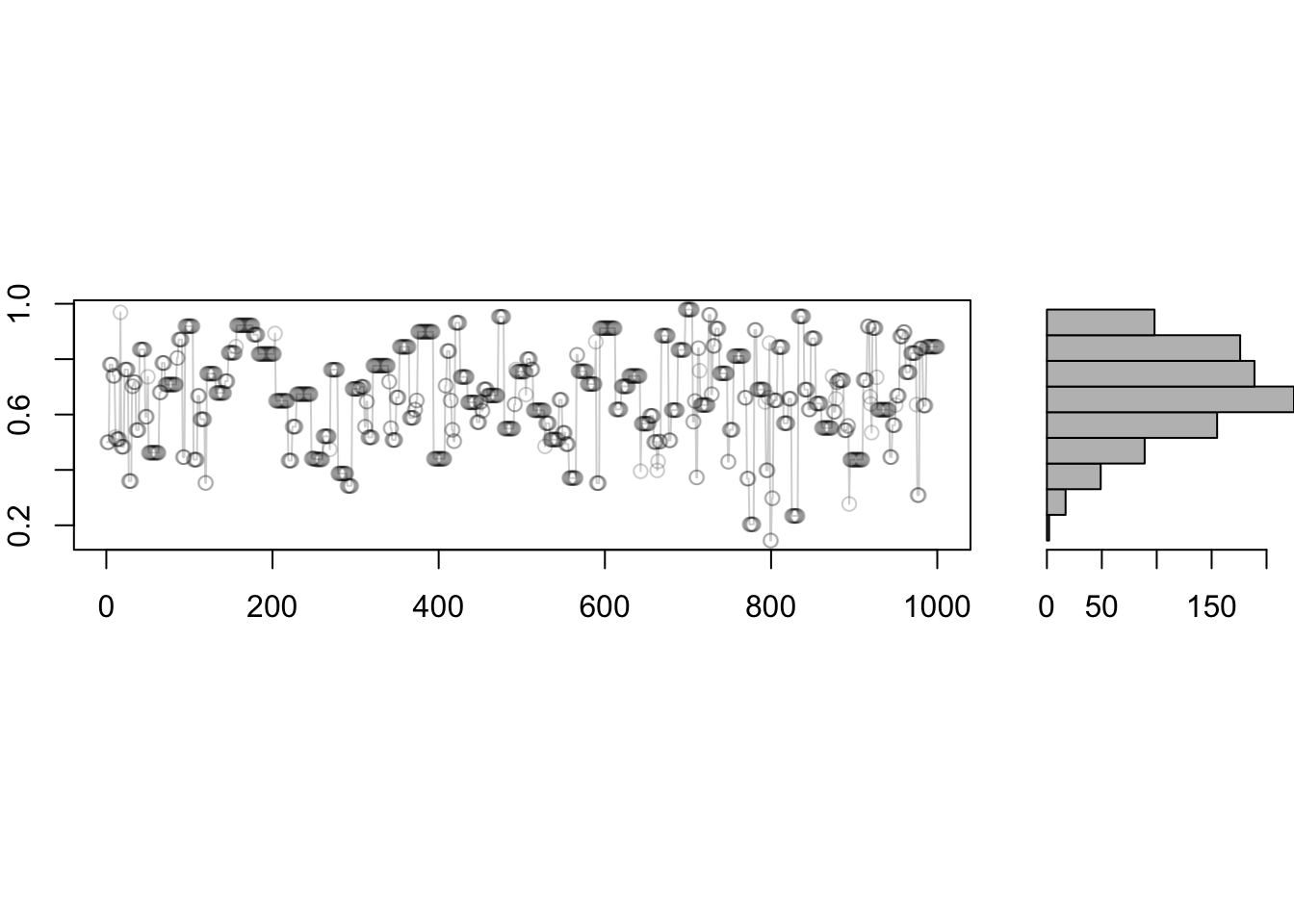
source("../blocks/plot_traces_and_hist.R")
samples = mcmc_mixture(gamma_beta_binomial, 0.5,  1000)
plot_traces_and_hist(samples)- 1
- Flip a coin.
- 2
- Use kernel corresponding to the coin flip outcome.

Mathematical notation for kernel mixtures
- Instead of using \(K_1\) and \(K_2\) with equal probability…
- …let \(\rho_1\) denote the probability to use \(K_1\),
- …and \(\rho_2 = 1 - \rho_1\).
Expression for the mixture of the two kernels: \[K_\text{mix}(x' | x) = \sum_{i=1}^2 \rho_i K_i(x' | x). \]
Invariance result
Mixtures preserve invariance
Proposition: if each \(K_i\) is \(\pi\)-invariant, then their mixture is \(\pi\)-invariant.
Question: can you prove this result? Convince yourself at the same time that the argument crucially depends on \(\rho_i\) not varying with the current state.
\[\begin{align*} \sum_x \pi(x) K(x' | x) &= \sum_x \pi(x) \sum_i \rho_i K_i(x' | x) \;\;\text{(def of mixture)} \\ &= \sum_i \rho_i \sum_x \pi(x) K_i(x' | x) \\ &= \sum_i \rho_i \pi(x') \;\;\text{(invariance of each $K_i$)} \\ &= \pi(x') \sum_i \rho_i \\ &= \pi(x') \;\;\text{($\rho_i$ are probabilities)}. \\ \end{align*}\]
Methodological application
Question: would it be a good idea to use the current state to adapt the mixture proportion (i.e., using \(\rho_i(x)\) instead of \(\rho_i\))?
- Yes, it would improve mixing.
- Yes, it would reduce the running time.
- No, it would break irreducibility.
- No, it would break invariance.
- None of the above.
No, it would break \(\pi\)-invariance.
Let us rewrite the first few steps of the above invariance argument, with \(\rho_i(x)\) instead of \(\rho\), until the argument breaks down: \[\begin{align*} \sum_x \pi(x) K(x' | x) &= \sum_x \pi(x) \sum_i \rho_i(x) K_i(x' | x) \;\;\text{(def of mixture)} \\ &\neq \sum_i \rho_i(x) \sum_x \pi(x) K_i(x' | x), \\ \end{align*}\] where the last line does not make sense, i.e. \(\rho_i(x)\) now depends on \(x\), so we cannot rearrange the sums in a way that makes it possible to invoke invariance of the \(K_i\). Can you identify an explicit counter example?