source("../../solutions/simple.R")

doomsday_model = function() {
  x = simulate(Unif(0, 5))
  observe(0.06, Unif(0, x))
  return(x)
}

posterior(doomsday_model, 100000)
[1] 1.105568We will write many Stan models in the coming weeks, so we will cover here the key concepts needed to write in Stan. Similarities with simPPLe will help in this process.
Let us revisit the Doomsday model, which we wrote in simPPLe as follows:

source("../../solutions/simple.R")
doomsday_model = function() {
x = simulate(Unif(0, 5))
observe(0.06, Unif(0, x))
return(x)
}
posterior(doomsday_model, 100000)[1] 1.105568Recall the analytic answer that we computed in clicker questions was: \(\approx 1.117\).
Today we will re-write this model in Stan instead of simPPLe. The main difference is that:
simulate and observe will be denoted by ~ in Stan,data or parameters).First, put the following code into a file called doomsday.stan:
doomsday.stan
data block will be treated as observed.
parameters block will be treated as latent, i.e., unobserved.x is declared latent (i.e., inside a parameters block), Stan will know to treat this as the counterpart of simPPLe’s x = simulate(Unif(0, 5)).
y is declared observed (i.e., inside a data block), Stan will know to treat this as the counterpart of simPPLe’s observe(0.06, Unif(0, x)).
Question: How does Stan get the actual observed value \(y = 0.06\)?
Answer: When Stan gets called from R:
Running MCMC with 1 chain...

Chain 1 Iteration:      1 / 101000 [  0%]  (Warmup)
Chain 1 Iteration:   1001 / 101000 [  0%]  (Sampling)
Chain 1 Iteration:  51000 / 101000 [ 50%]  (Sampling)
Chain 1 Iteration: 101000 / 101000 [100%]  (Sampling)
Chain 1 finished in 0.9 seconds.
We can now compare the approximation provided by Stan:
fit variable mean median sd mad q5 q95 rhat ess_bulk ess_tail
lp__ -0.37 -0.12 0.64 0.14 -1.62 -0.02 1.00 19501 24505
x 1.11 0.55 1.25 0.65 0.07 4.01 1.00 19501 24505;uniform.To access the samples from a “fit” object when calling Stan, use:
xs = as.vector(fit$draws("x"))As a sanity check, let’s make sure all the samples are greater than the observed lower bound of \(0.06\):
min(xs)[1] 0.06001702Question: denote the samples output from Stan by \(X^{(1)}, X^{(2)}, \dots, X^{(M)}\). What formula should you use to approximate \(\mathbb{E}[g(X) | Y = y]\) based on the Stan output?
As in simple Monte Carlo, use \(\frac{1}{M} \sum_{m=1}^M g(X^{(m)})\).
Since the samples are equally weighted, this makes it simpler to create plots, e.g., for a histogram:
hist(xs)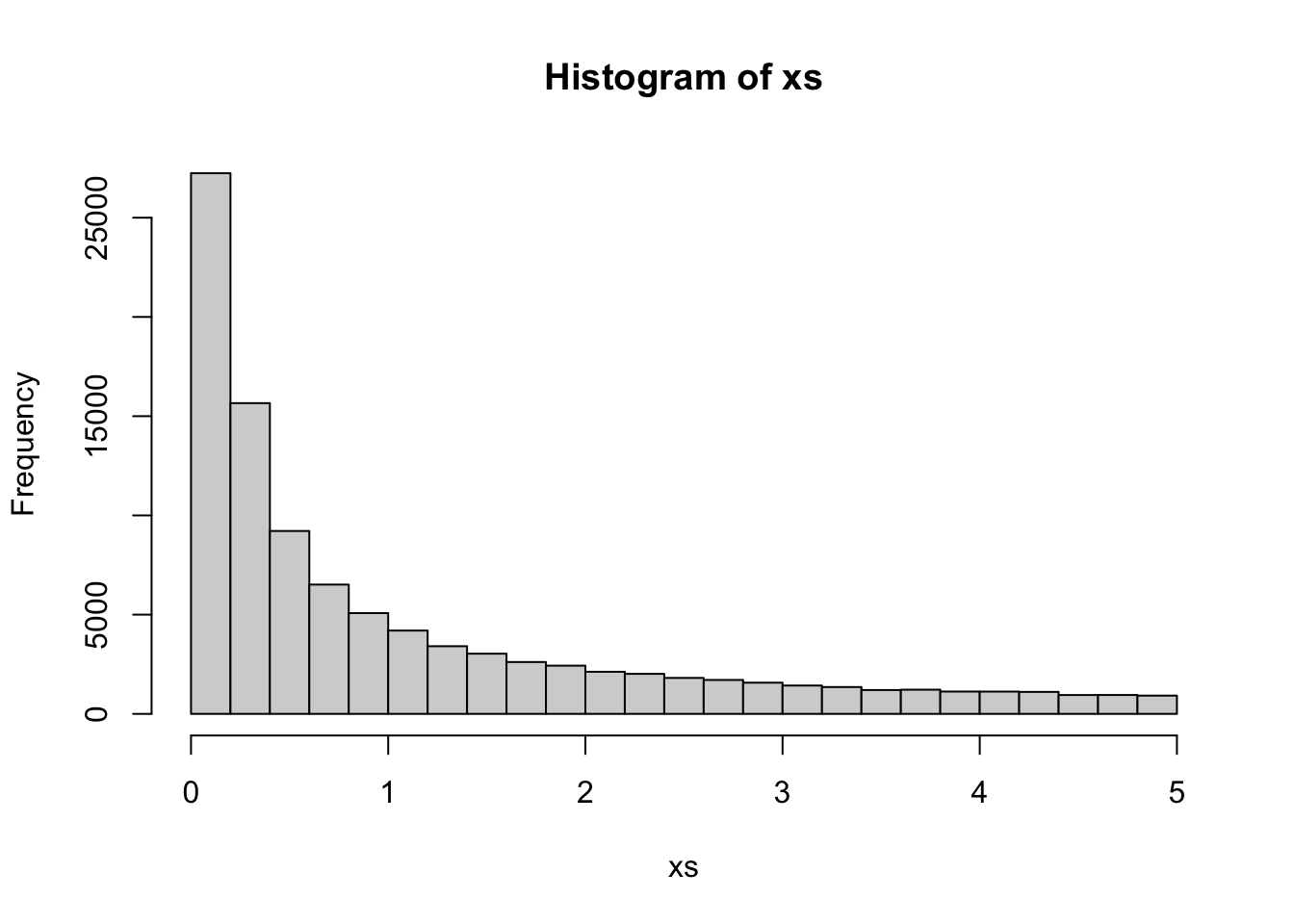
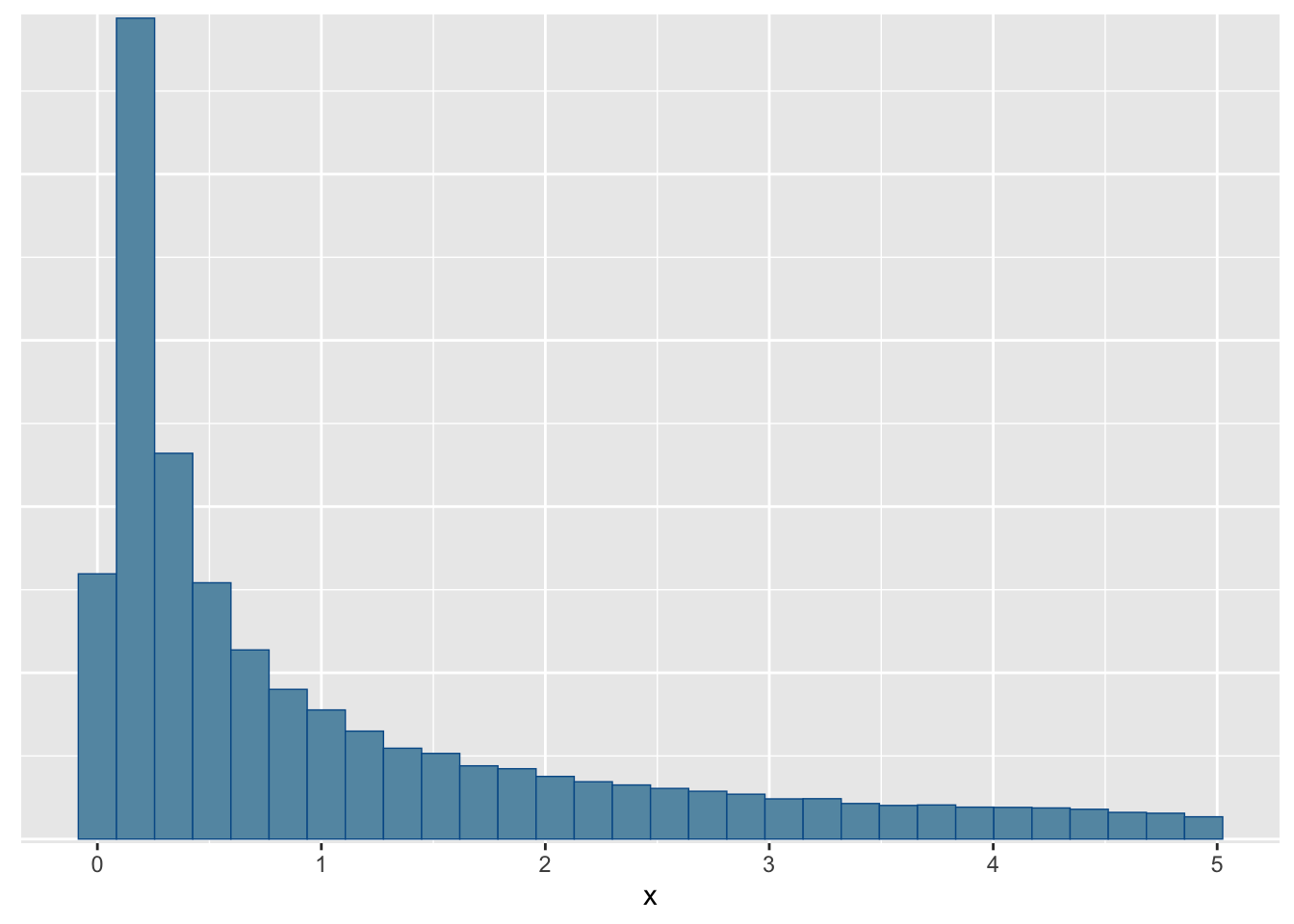
You can also use the bayesplot package which will be handy to create more complex plots from MCMC runs:
suppressPackageStartupMessages(library(bayesplot))
mcmc_hist(fit$draws(), par = c("x"))
`stat_bin()` using `bins = 30`. Pick better value with `binwidth`.