suppressPackageStartupMessages(library(cmdstanr))Custom bricks
Outline
Topics
- What to do when you need a distribution not in the Stan built-in library.
- Understanding why Stan (and most MCMC methods) represents the density in log-scale.
Rationale
Even though Stan has a long list of built-in distributions, you will eventually run into a situation where you need a distribution not in the list.
While learning how to do so, we will need to look more deeply at how Stan works under the hood.
Example
We will show how to implement the Kumaraswamy distribution in Stan. As of March 2024, it is not in Stan’s built-in library.

The Kumaraswamy distribution has density: \[f(x) = ab x^{a-1} (1 - x^a)^{b-1},\] where \(x \in (0, 1)\) and \(a, b\) are positive parameters.
Executive version
- In the
modelblock:- Use
target += [logarithm (base e) of the density] - Applying this to our Kumaraswamy example: \[\log(f(x)) = \log(a) + \log(b) + (a-1) \log(x) + (b-1) \log(1 - x^a).\]
- Use
- In the
parametersblock:- Make sure you enforce the support (here \(x \in (0, 1)\))
kumaraswamy.stan
- 1
- Support is enforced.
- 2
- Contribution of the Kumaraswamy log density added to the log joint density.
mod = cmdstan_model("kumaraswamy.stan")
fit = mod$sample(
seed = 1,
refresh = 0,
data = list(a = 2, b = 5),
chains = 1,
output_dir = "stan_out",
iter_sampling = 10000
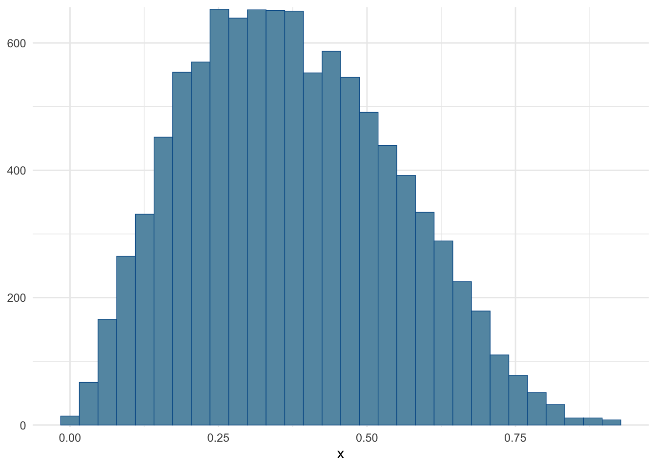
)Checking that the histogram roughly matches the one from the Wikipedia article (see top of page Figure, purple line).
suppressPackageStartupMessages(library(bayesplot))
suppressPackageStartupMessages(library(ggplot2))
mcmc_hist(fit$draws("x")) + theme_minimal()
Explanation
Log-scale computation
Question: why is Stan computing the logarithm of \(\gamma(x)\)?
Key fact: Stan, like most numerical methods, uses double-precision floating point approximation of real numbers.
- Suppose you have 500 observations.
- Each has a likelihood of about \(1/10\).
- What is the joint likelihood?
likelihood = 1.0
for (i in 1:500) {
  likelihood = likelihood * (1/10)
}
likelihood
[1] 0Question: Why does R return zero?
CautionClick for answer
- Because \((1/10)^{500}\) is smaller than the smallest positive number representable in double precision (\(\approx 10^{-300}\))
- So it gets rounded to zero.
- This is called an underflow.
Log-scale computation: let us say we store instead the log-likelihood:
loglikelihood = log(1.0)
for (i in 1:500) {
  loglikelihood = loglikelihood + log(1/10)
}
loglikelihood
[1] -1151.293500*log(1/10)[1] -1151.293- We have avoided the underflow issue!
- That’s why a Stan program computes \(\log \gamma(x)\) instead of \(\gamma(x)\).
Encapsulation into a function
If you are using a custom density for several variables, encapsulate it into a function:
kumaraswamy_as_function.stan
- 1
-
The
functionblock allows you to create custom functions. See the Stan documentation for more details. - 2
-
For Stan to pick up your function in its
~syntax, you must use the special suffix_lpdffor your function name, which stands for “log probability density function.” - 3
-
Then you can use your distribution name using
~as usual (notice we do not include the_lpdfwhen we make such call). From this it is apparent that Stan’s~notation is just a shortcut fortarget += distributionName_lpdf(...).
mod = cmdstan_model("kumaraswamy_as_function.stan")
fit = mod$sample(
  seed = 1,
  refresh = 0,
  data = list(a = 2, b = 5),
  chains = 1,
  output_dir = "stan_out",
  iter_sampling = 10000
)