Posterior distributions
Outline
Topics
- Notion of posterior distribution.
- Examples
- How to use a posterior?
Rationale
The posterior distribution appears in the second step of the Bayesian Recipe and is therefore encountered (at least implicitly) in all full Bayesian problems.
Definition
The conditional PMF of the unknowns \(X\) given the observation \(Y\) is called the posterior PMF.1
Notation
We use \(\pi(x) = \mathbb{P}(X = x | Y = y)\) for the posterior PMF.
Recall:
\[\pi(x) = \frac{\gamma(x)}{Z},\]
where \(\gamma(x) = \mathbb{P}(X = x, Y = y)\) is the un-normalized posterior and \(Z = \mathbb{P}(Y = y)\) is the normalization constant.
Examples
Example 1: coins in a bag
Visualization of the prior PMF and how it arises from the decision tree and random variable \(X\) (showing 3 flips instead of 4):
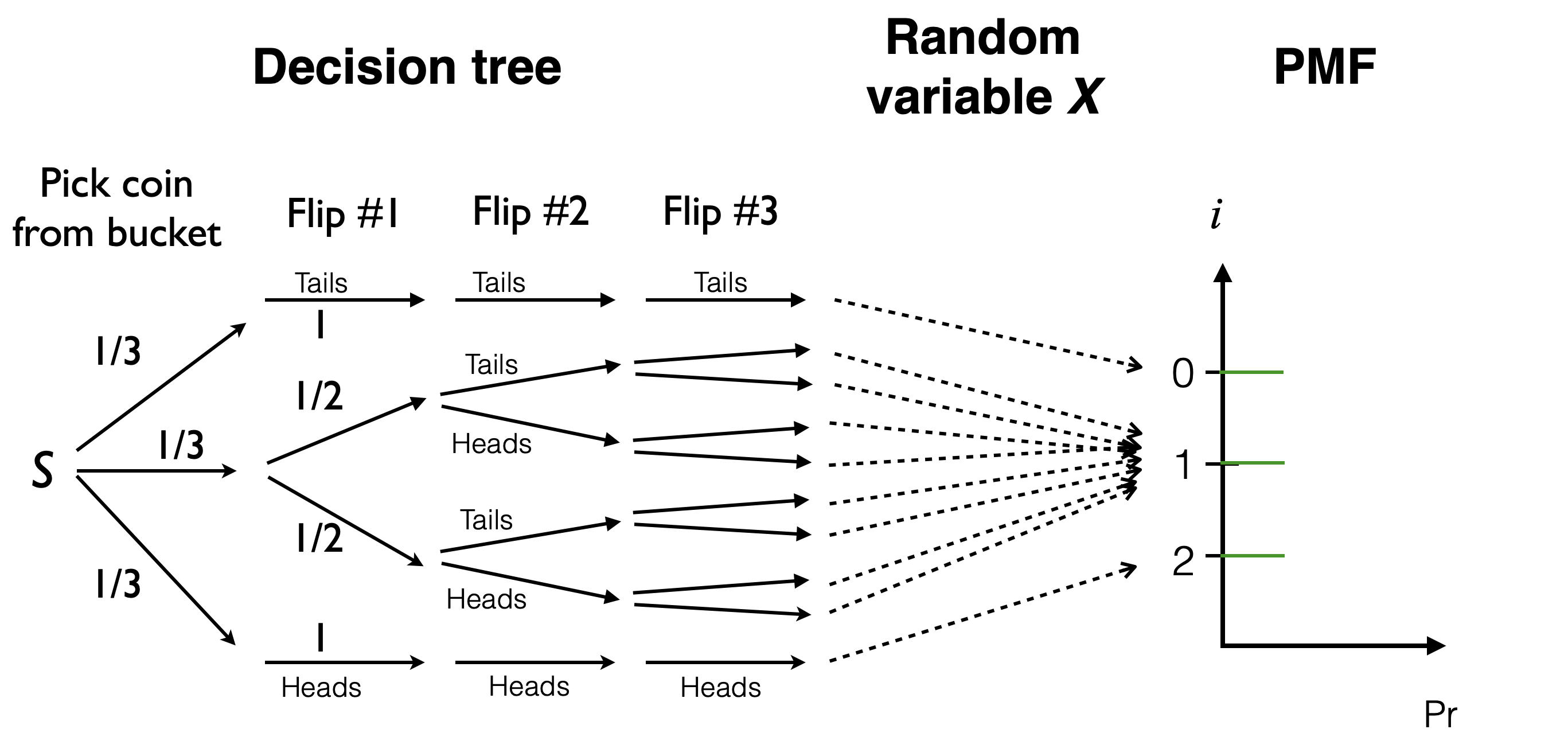
- Recall that the probability of each path is the product of the edge labels.
Visualization of the posterior PMF and how it arises from the decision tree and random variable \(X\):
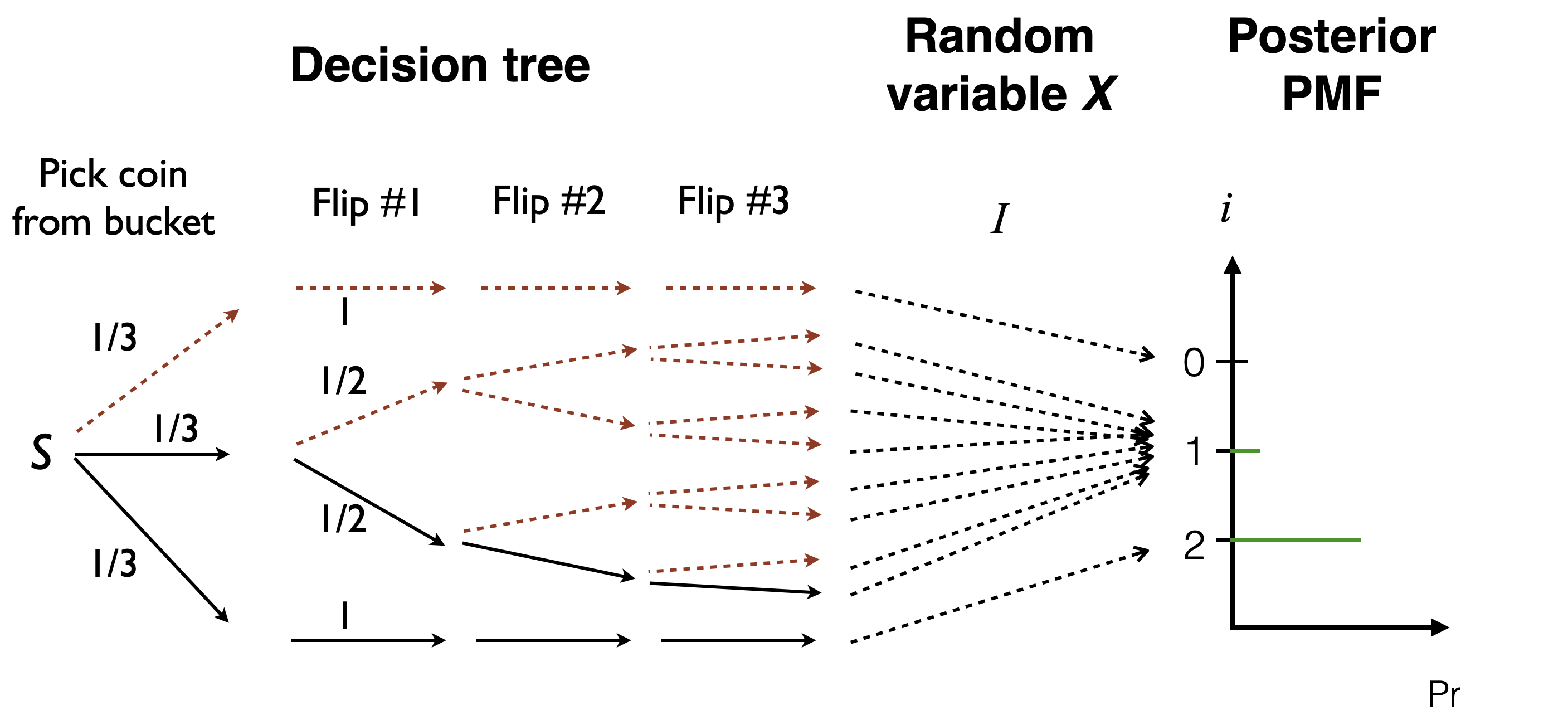
- Recall we zero out the contribution of the paths not compatible with the observation (Heads, Heads, Heads).
- This gives a list of numbers that do not sum to one, so we renormalize them.
Example 2: rocket insurance
You will construct prior and posterior PMFs in question 2 of this week’s exercises.
What to do with a posterior?
- Show a visualization (posterior PMF).
- Compute a summary of the PMF:
- point estimate: single “best guess”, or
- a credible region: a set of “guesses”.
- More generally: decision theory / Step 3 of the Bayesian Recipe.
Footnotes
if the unknown quantity is continuous, the posterior will be expressed using a density. A term that captures both the continuous and discrete cases is “distribution” i.e. “posterior distribution”.↩︎