Mixtures

Outline

Topics

• Mathematical definition of mixtures
• Implementation in Stan

Rationale

Mixtures are motivated by cases where you believe the data is composed of two or more distinct sub-populations.

One use of mixtures is to figure out, for each data point, from which sub-population it comes from.

Beyond the sub-population example, mixtures are also used to get more flexible distribution families.

Example: detection of random guessing

• We look at a dataset from Albert and Hu, 2020.
• We have scores for 30 students on a test.
• The test has 20 questions.
• All questions are TRUE/FALSE with same weight.
• Every student attempted every question.

suppressPackageStartupMessages(require(rstan))
suppressPackageStartupMessages(require(ggplot2))
suppressPackageStartupMessages(require(dplyr))
suppressPackageStartupMessages(require(bayesplot))

data = read.csv(url("https://github.com/UBC-Stat-ML/web447/raw/main/data/ScoreData.csv"))
rmarkdown::paged_table(data)

plot(data$Score,
      ylim = c(0, 20),
      xlab = "Student index", 
      ylab = "Score (out of 20 questions)")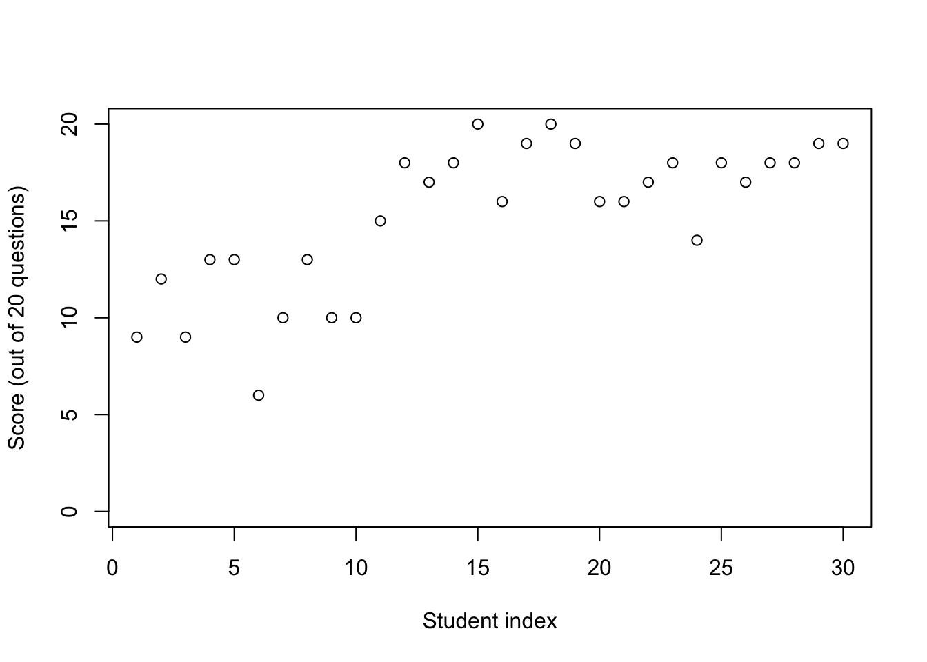

• Notice a cluster of students with scores around 50%,
• and a second cluster with much better scores.
• Hypothesis: some students answered completely at random.

Simplified problem

• Suppose first that we have the score for only one student.
• E.g.: first one, who got 9/20.
• You want a model to put a probability on: “is this student is guessing at random?”
  • Real application: analysis of clicker scores where grade is participation-based.

Mathematical model

• Start with the data: \(Y\), an integer between 0 and 20.

Question: what is a good choice of likelihood?

Click for hint

We can write \(Y = Y_1 + Y_2 + \dots + Y_{20}\), where \(Y_j\) is a Bernoulli for the score of question \(j\).

Click for choices

1. Normal.
2. Binomial.
3. Discrete uniform.
4. Continuous uniform.
5. None of the above.

Click for answer

Since \(Y\) is a sum of Bernoullis, if we assume that the questions are independent, then this suggests a binomial likelihood family.

• The parameters of the likelihood depend on whether the student is guessing or not
  • Let \(G\) denote an indicator on guessing, i.e.:
    • \(G = 1\): guessing,
    • \(G = 0\): not guessing, i.e., trying at the best of their ability.

Question: what is a good choice of prior on \(G\)?

Click for choices

1. \(\mathcal{N}(0, 1)\)
2. \({\mathrm{Unif}}(0, 1)\)
3. \({\mathrm{Bern}}(1/3)\)
4. \({\mathrm{Exp}}(1/100)\)
5. None of the above.

Click for answer

Since \(G\) can only take values \(0\) or \(1\), the prior has to be taken from the Bernoulli family.

We put \(1/3\) to model a prior belief that students guessing at random will be a minority.

• The likelihood given \(G = 1\) (guessing) is easy: \[Y \sim {\mathrm{Binom}}(20, 0.5).\]
• The likelihood given \(G = 0\) (trying at the best of their ability) is slightly trickier:
  • what is “the best of their ability”?
  • Bayesian recipe: treat it as an unknown ability parameters \(A\)

Full model:

\[\begin{align*} A &\sim {\mathrm{Unif}}(0, 1) \\ G &\sim {\mathrm{Bern}}(1/3) \\ Y &\sim {\mathrm{Binom}}(20, 0.5 G + A(1-G)). \end{align*}\]

Marginalization

• Stan does not support discrete latent random variables like \(G\)
• Therefore we use Rao-Blackwellization:
  • Joint distribution before Rao-Blackwellization: \[\gamma(a, g, y) = p(a) p(g) p(y|a, g).\]
  • Joint distribution after Rao-Blackwellization: \[\begin{align*} \gamma(a, y) &= \sum_{g=0}^1 \gamma(a, g, y) \\ &= \sum_{g=0}^1 p(a) p(g) p(y|a, g) \\ &= p(a) \sum_{g=0}^1 p(g) p(y|a, g) \\ &= \underbrace{p(a)}_\text{(a)} \underbrace{\left( \underbrace{p(g=1) p(y|a, g=1)}_\text{(b)} + \underbrace{p(g=0) p(y|a, g=0)}_\text{(c)} \right)}_\text{(d)}. \end{align*}\]

Question: match-up (a)-(d) with the labelled statements in the Stan code below.

Click for choices

1. (a) <-> ③, (b) <-> ②, (c) <-> ①, (d) <-> ⑤,
2. (a) <-> ③, (b) <-> ①, (c) <-> ②, (d) <-> ⑤,
3. (a) <-> ③, (b) <-> ②, (c) <-> ①, (d) <-> ④,
4. (a) <-> ③, (b) <-> ①, (c) <-> ②, (d) <-> ④,
5. None of the above.

Click for answer

The matching:

(a) <-> ③, (b) <-> ①, (c) <-> ②, (d) <-> ④,

is the correct answer.

data {
  int<lower=0, upper=20> score;
}

parameters {
  real<lower=0, upper=1> ability;
}

transformed parameters {
1  real complete_likelihood_guessing
    = 1.0/3 * exp(binomial_lpmf(score | 20, 0.5)); 
2  real complete_likelihood_non_guessing
    = 2.0/3 * exp(binomial_lpmf(score | 20, ability)); 
}

model {
3  ability ~ uniform(0, 1);
4  target +=
    log(complete_likelihood_guessing + complete_likelihood_non_guessing); 
}

generated quantities {
5  real guessing_probability =
    complete_likelihood_guessing / (complete_likelihood_guessing + complete_likelihood_non_guessing);
}

1

Stan statement 1 (used in clicker question)

2

Stan statement 2

3

Stan statement 3

4

Stan statement 4

5

Stan statement 5

Re-instatiation

• We care about the posterior mean of \(G\), \(\mathbb{E}[G | Y = y]\)…
• …but we have marginalized \(G\) 🙁
• To compute the posterior mean, we first use the law of total expectation: \[\mathbb{E}[G | Y] = \mathbb{E}[{\color{red} \mathbb{E}[G | A, Y]} | Y],\]
• Let us look at the part in red, and see how we can compute it at every MCMC iteration based on the current value of \(A^{(m)}\)…
  • Using the fact the mean of a Bernoulli is the probability that it takes value 1: \[\mathbb{E}[G | A, Y] = \mathbb{P}(G = 1 | A, Y).\]
  • By Bayes rule (noting that a conditional probability like \(\mathbb{P}(\cdot | A)\) is a probability): \[\mathbb{P}(G = 1 | A, Y = y) = \frac{\mathbb{P}(G = 1, Y = y | A)}{\mathbb{P}(G = 0, Y = y | A) + \mathbb{P}(G = 1, Y = y | A)}.\]
  • This is what gets computed in statement ⑤ in the above Stan code.
• Now, recall from the LLN for Markov chains gives us condition so that for a test function \(h\), we have that the Monte Carlo samples, \(A^{(1)}, A^{(2)}, \dots, A^{(M)}\) satisfy, \[\frac{1}{M} \sum_{m=1}^M h(A^{(m)}) \to \mathbb{E}[h(A) | Y = y],\] with probability one.
• Therefore from taking \(h(A^{(m)}) = \mathbb{P}(G = 1 | A^{(m)}, Y = y)\), we obtain, \[\frac{1}{M} \sum_{m=1}^M \mathbb{P}(G = 1 | A^{(m)}, Y = y) \to \mathbb{E}[G | Y = y],\] with probability one.

Testing the model

Probably guessing: feeding a score of 9 out of 20, we get:

fit = sampling(
  students_guessing_simplified,
  seed = 1,
  refresh = 0,
  data = list(score = 9)       
)

mean(extract(fit)$guessing_probability)

[1] 0.613919

Probably not guessing: feeding a score of 19 out of 20, we get:

fit = sampling(
  students_guessing_simplified,
  seed = 1,
  refresh = 0,
  data = list(score = 19)      
)

mean(extract(fit)$guessing_probability)

[1] 9.302208e-05

What is the key limitation of this approach?

Click for answer

The student could have a low score because the questions were too difficult!

With some assumptions (unimodality of the students abilities) we can avoid this limitation.

Full model: getting rid of key limitation

• Idea: use a hierarchical model!
• Random variables that are student-specific:
  • \(Y_i \sim {\mathrm{Binom}}(20, 0.5 G_i + A_i (1 - G_i)).\)
  • \(A_i \sim {\mathrm{Beta}}(\mu, S)\)
  • \(G_i \sim {\mathrm{Bern}}(F)\)
• Random variables that are global:
  • Population fraction that are guessing: \(F \sim {\mathrm{Unif}}(0, 1)\),
  • Population parameters for the abilities:
    • \(\mu \sim {\mathrm{Unif}}(0, 1)\)
    • \(S \sim {\mathrm{Exp}}(1/100)\).
• Stan implementation:

data {
  int n_students; 
  array[n_students] int<lower=0, upper=20> scores; 
}

parameters {
  real<lower=0, upper=1> fraction_guessing;
  real<lower=0, upper=1> non_guessing_population_mean;
  real<lower=0> non_guessing_population_spread;
  vector<lower=0, upper=1>[n_students] abilities;
}

transformed parameters {
  vector[n_students] complete_loglikelihood_guessing; 
  vector[n_students] complete_loglikelihood_non_guessing; 
  for (i in 1:n_students) {
    complete_loglikelihood_guessing[i]     
      = log(fraction_guessing) + binomial_lpmf(scores[i] | 20, 0.5); 
    complete_loglikelihood_non_guessing[i] 
      = log1p(-fraction_guessing) + binomial_lpmf(scores[i] | 20, abilities[i]);
  }
}

model {
  fraction_guessing ~ uniform(0, 1);
  non_guessing_population_mean ~ uniform(0, 1);
  non_guessing_population_spread ~ exponential(1.0/100);
  for (i in 1:n_students) {
    abilities[i] ~ beta_proportion(non_guessing_population_mean, non_guessing_population_spread);
    target += 
      log_sum_exp(complete_loglikelihood_guessing[i], complete_loglikelihood_non_guessing[i]);
  }
}

generated quantities {
  vector[n_students] guessing_probabilities = inv_logit(complete_loglikelihood_guessing - complete_loglikelihood_non_guessing);
  real predictive_score_non_guessing = 20 * beta_proportion_rng(non_guessing_population_mean, non_guessing_population_spread);
}

fit = sampling(
  students_guessing,
  seed = 1,
  refresh = 0,
  data = list(
            n_students = length(data$Score),
            scores = data$Score
          )                  
)

Credible intervals and posterior medians: 90% (thick lines) and 50% (thin lines)

mcmc_intervals(fit, regex_pars = c("guessing_probabilities.*")) + 
  theme_minimal() + 
  scale_x_continuous(limits = c(0, 1))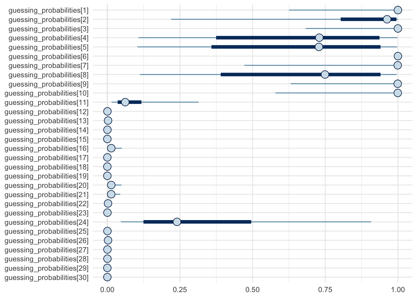 

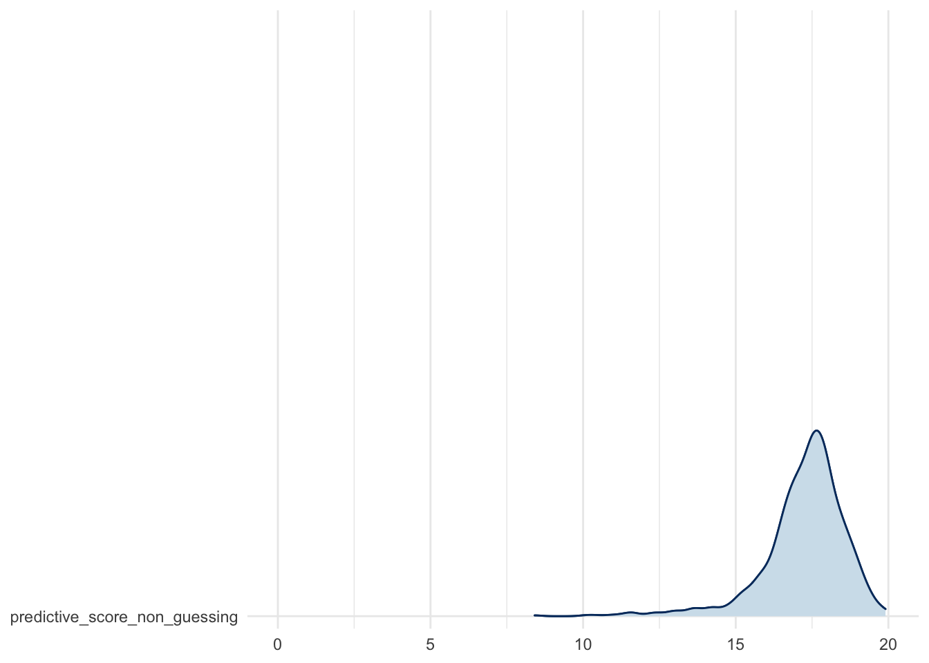
Predictive score distribution: for the non guessing sub-population…

mcmc_areas_ridges(fit, regex_pars = c("predictive_score_non_guessing*")) + 
  theme_minimal() + 
  scale_x_continuous(limits = c(0, 20))