Practice questions (Quiz 2)

Caution

Page under construction: information on this page may change.

Outline

Topics

Representative example of questions to prep for Quiz 2.

Important note

Make sure to practice the similar page for Quiz 1 since quiz 2 will cover that material as well.

Libraries needed to run the example below

suppressPackageStartupMessages(require(rstan))

Model construction

Consider the following setup

You have a cohort of 15 unemployed persons who are all starting a job search process at the same time.
For each participant, you have collected 2 covariates: their age and their number of years of education.
You contact the participants each day for 10 days and record the day they secured a new job.
At the end of your study, 3 of the participants are still looking for a job.

Using the `~` notation

Define a Bayesian model to handle this dataset. Introduce all random variables, and specify for each its data type, if it observed or not.

Click for answer

The random variables are:

Let \(y_1, y_2, \dots, y_{12}\) denote the job search times for the 12 participants who found a job in the study interval (10 days). These variables are observed.
Let \(y_{13}, y_{14}, y_{15}\) denote the job search times for the other 3 participants. These variables are latent.
Let \(f_i\) denote an indicator variable equal to one iff participant \(i\) found a job in the 10 days period, \(i \in \{1, 2, \dots, 15\}\). These variables are observed.
Let \(x_{i,j}\), \(i \in \{1, 2, \dots, 15\}, j \in \{1, 2\}\) denote the age (\(j=1\)) or years of education (\(j=2\)) for participant \(i\). These variables are observed.
Set \(x_{i,0} = 1\) to simplify the notation for the intercept.
Let \(\theta_0\) denote and intercept parameter, \(\theta_1, \theta_2\), slope parameters for the age and number of years of education. These variables are latent.

One potential model is: \[\begin{align*} \theta_j &\sim \mathcal{N}(0, 100), \\ \phi &\sim {\mathrm{Exp}}(1/100), \\ \mu_i &= \exp\left(\sum_{j=0}^3 x_{i,j} \theta_j\right) \\ y_i &\sim {\mathrm{NegBinom}}\left(\mu_i, \phi\right), \\ f_i &= \mathbb{1}[y_i \le 10]. \end{align*}\]

Rao-blackwellization

Write the joint density of the model in the last part, before and after Rao-Blackwellization. You can introduce symbols for densities and CDFs, for example leave the density of the exponential as \(p_\text{Exp}(x; \lambda),\) and similarly use \(F_\text{Name}(\cdot; \cdot)\) to denote CDFs.

Click for answer

Before Rao-Blackwellization, we have:

\[\begin{align*} p(\phi, \theta_1, &\dots, \theta_3, y_1, y_2, \dots, y_{15}, f_1, f_2, \dots, f_{15}) = \\ &p_\text{Exp}(\phi; 1/100) \left( \prod_{j=0}^2 p_\text{Norm}(\theta_j; 0, 100) \right) \\ &\left( \prod_{i=1}^{15} p_\text{NB}\left(y_i; \mu_i, \phi\right) p_\text{Bern}(f_i; \mathbb{1}[y_i \le 10]) \right). \end{align*}\]

Rao-Blackwellizing the above: \[\begin{align*} \sum_{y_{13}=0}^\infty \sum_{y_{14}=0}^\infty \sum_{y_{15}=0}^\infty p(\phi, \theta_1, &\dots, \theta_3, y_1, y_2, \dots, y_{15}, f_1, f_2, \dots, f_{15}) = \\ &p_\text{Exp}(\phi; 1/100) \left( \prod_{j=0}^2 p_\text{Norm}(\theta_j; 0, 100) \right) \\ &\left( \prod_{i=1}^{12} p_\text{NB}\left(y_i; \mu_i, \phi\right) p_\text{Bern}(f_i; \mathbb{1}[y_i \le 10]) \right) \\ & \sum_{y_{13}=0}^\infty \sum_{y_{14}=0}^\infty \sum_{y_{15}=0}^\infty \left( \prod_{i=13}^{15} p_\text{NB}\left(y_i; \mu_i, \phi\right) p_\text{Bern}(f_i; \mathbb{1}[y_i \le 10]) \right) \\ =&p_\text{Exp}(\phi; 1/100) \left( \prod_{j=0}^2 p_\text{Norm}(\theta_j; 0, 100) \right) \\ & \left( \prod_{i=1}^{12} p_\text{NB}\left(y_i; \mu_i, \phi\right) p_\text{Bern}(f_i; \mathbb{1}[y_i \le 10]) \right) \\ & \prod_{i=13}^{15} \left( 1 - F_\text{NB}\left(10; \mu_i, \phi\right) \right). \end{align*}\] Where in the first equality, we “pushed the sums inside” since the first three groups of factors do not have the sums’ arguments in them, \(y_{13}, y_{14}, y_{15}\).

The second equality is explained in more details below (showing just the part that gets simplified to keep notation shorter): \[\begin{align*} \sum_{y_{13}=0}^\infty & \sum_{y_{14}=0}^\infty \sum_{y_{15}=0}^\infty \left( \prod_{i=13}^{15} p_\text{NB}\left(y_i; \mu_i, \phi\right) p_\text{Bern}(f_i; \mathbb{1}[y_i \le 10]) \right) \\ &= \prod_{i=13}^{15} \left( \sum_{y_i = 0}^\infty p_\text{NB}\left(y_i; \mu_i, \phi\right) p_\text{Bern}(f_i; \mathbb{1}[y_i \le 10]) \right) \\ &= \prod_{i=13}^{15} \left( \sum_{y_i = 0}^\infty p_\text{NB}\left(y_i; \mu_i, \phi\right) (1 - \mathbb{1}[y_i \le 10]) \right) \\ &= \prod_{i=13}^{15} \left( 1 - \sum_{y_i = 0}^\infty p_\text{NB}\left(y_i; \mu_i, \phi\right) \mathbb{1}[y_i \le 10] \right) \\ &= \prod_{i=13}^{15} \left( 1 - F_\text{NB}\left(10; \mu_i, \phi\right) \right). \end{align*}\]

The steps above are justified as follows:

From line 1 to 2: associativity of addition and multiplication (for the same reason as e.g., \(\sum_i \sum_j a_i b_j = (\sum_i a_i)(\sum_j b_j)\) for any \(a_i\), \(b_j\)).
From line 2 to 3: using the fact that \(f_i = 0\) for \(i \in \{13, 14, 15\}\), and that \(p_\text{Bern}(0; p) = (1 - p)\).
From line 3 to 4: using the fact \(p_\text{NB}\) is a PMF and hence sums to one.
From line 4 to 5: using the definition of a CDF.

Model debugging

Let:

\(C(y)\) denote a 99% credible interval computed from data \(y\).
Let \(y\) and \(\check y\) denote a real and synthetic (simulated) data respectively.

Suppose you observed the following:

\(y_n \notin C(y_{\backslash n})\)
\(\check y_n \notin C(\check y_{\backslash n})\)
On both synthetic and real data, trace plots and ESS both look good.
You replicated these experiments several times and always get the same results.

What would you do next? Justify your answer.

Click for answer

Referring to the workflow notes on goodness of fit and software checking, we have:

From 3, we can exclude “slow mixing.”
From 4, we can exclude “bad luck.”
From 2, we therefore know there has to be a software defect (bug).
Since 1 can be caused by either a software defect or a gross mis-specification, this item does not provide additional information.

Therefore, the next step would be to fix the bug(s).

Normalization constant

Consider the Bayesian model:

\[\begin{align*} X &\sim {\mathrm{Exp}}(1/100) \\ Y &\sim {\mathrm{Poisson}}(X). \end{align*}\]

When using MCMC, will the output change if, for \(x > 0\)…

You used \(\check f(x) = \exp(-(1/100) x)\) instead of \(f(x) = (1/100) \exp(-(1/100) x)\) for the prior?
You used \(\hat f(y|x) = x^y / y!\) instead of \(f(y|x) = \exp(-x) x^y / y!\) for the likelihood?

Click for answer

For 1, the output will not change as the MH ratio with \(\check f(x)\) is:

\[ \check r = \frac{\gamma(\tilde x)}{\gamma(x)} = \frac{ \exp(-(1/100) \tilde x) f(y|\tilde x)}{ \exp(-(1/100) \tilde x) f(y|x)} \]

whereas for \(f(x)\) we get:

\[ r = \frac{\gamma(\tilde x)}{\gamma(x)} = \frac{ (1/100) \exp(-(1/100) \tilde x) f(y|\tilde x)}{ (1/100) \exp(-(1/100) \tilde x) f(y|x)} \] So we see the \((1/100)\) factors on numerator and denominator cancel and we have \(r = \check r\).

For 2, the output would change since for \(\hat f(y|x)\) we have:

\[ \hat r = \frac{\gamma(\tilde x)}{\gamma(x)} = \frac{ f(\tilde x) \tilde x^y / y! }{ f(x) x^y / y! } \] whereas for \(f(x)\) we get:

\[ r = \frac{\gamma(\tilde x)}{\gamma(x)} = \frac{ f(\tilde x) \exp(-\tilde x) \tilde x^y / y! }{ f(x) \exp(-x) x^y / y! } \]

and hence \(r = \hat r \exp(x - \tilde x)\) so \(r\) and \(\hat r\) are not equal.

Intervals

Suppose you see the following output from a Stan MCMC fit object:

Inference for Stan model: anon_model.
1 chains, each with iter=2000; warmup=1000; thin=1; 
post-warmup draws per chain=1000, total post-warmup draws=1000.

            mean se_mean   sd  2.5%   25%   50%   75% 97.5% n_eff Rhat
slope       0.42    0.00 0.04  0.34  0.40  0.42  0.45  0.51   719    1
sigma       0.24    0.00 0.04  0.18  0.21  0.24  0.27  0.33   639    1
prediction  0.64    0.01 0.27  0.14  0.47  0.64  0.81  1.20  1023    1
lp__       21.32    0.06 1.04 18.46 20.94 21.62 22.09 22.36   331    1

Samples were drawn using NUTS(diag_e) at Thu Mar 14 14:41:50 2024.
For each parameter, n_eff is a crude measure of effective sample size,
and Rhat is the potential scale reduction factor on split chains (at 
convergence, Rhat=1).

Report a 80% confidence interval to capture the Monte Carlo error for the posterior mean of the prediction parameter.

Some of the following will be helpful in answering that question:

qnorm(0.8)

[1] 0.8416212

qnorm(0.9)

[1] 1.281552

qnorm(0.95)

[1] 1.644854

Report a 50% credible interval for the prediction parameter. You can ignore Monte Carlo error in this sub-question.

Click for answer

We need to split the \(1-20\%\) into the two tails, hence we are looking for the 10% tail.

The radius of the interval is therefore:

0.01 * qnorm(0.9)

[1] 0.01281552

Hence the interval is \([0.64 \pm 0.01]\).

A quantile-based credible interval gives \([0.47, 0.81]\).

Bias and consistency

Let \(\hat G_M\) denote a Monte Carlo estimator based on \(M\) iterations, providing an approximation for an intractable expectation, \(g^* = \mathbb{E}_\pi[g(X)]\).

Define the notion of bias.
Define the notion of consistency.
In the context of Monte Carlo methods, what is more important, a bias of zero (unbiasness) or consistency? Why?

Click for answer

\(\operatorname{Bias}(\hat G_M, g^*) = \mathbb{E}[\hat G_M] - g^*\).
\(\hat G_M \to g^*\).¹
Consistency is more important. Consistency means that the error decreases as \(M\) increases. In contrast, even if a method is unbiased, it still leads to error due to its variance.

Stan-based prediction

Consider the code you wrote in Exercise 7 to perform Bayesian linear regression on galaxy distances and velocities:

data {
  int<lower=0> N; // number of observations
  vector[N] xs;   // independent variable
  vector[N] ys;   // dependent variable
}

parameters {
  real slope;
  real<lower=0> sigma;
}

model {
  // prior
  slope     ~ student_t(3, 0, 100);
  sigma     ~ exponential(0.001);

  // likelihood
  ys ~ normal(slope*xs, sigma);
}

How would you modify this code to predict the velocity of a galaxy at distance 1.5? Hint: use the function normal_rng(mean, sd) to generate a normal random variable with the provided mean and standard deviation parameters.

Click for answer

data {
  int<lower=0> N; // number of observations
  vector[N] xs;   // independent variable
  vector[N] ys;   // dependent variable
}

parameters {
  real slope;
  real<lower=0> sigma;
}

model {
  // prior
  slope     ~ student_t(3, 0, 100);
  sigma     ~ exponential(0.001);

  // likelihood
  ys ~ normal(slope*xs, sigma);
}

generated quantities {
  real prediction = normal_rng(slope*1.5, sigma);
}

suppressPackageStartupMessages(require(ggplot2))
suppressPackageStartupMessages(require(dplyr))

df = read.csv(url("https://github.com/UBC-Stat-ML/web447/raw/0d6eaa346d78abe4cd125e8fc688c9074d6331d9/data/hubble-1.csv")) %>%
  rename(distance = R..Mpc.) %>%
  rename(velocity = v..km.sec.)
df$velocity = df$velocity/1000

Run the above program using (the part below you are not expected to memorize):

fit = sampling(
  hubble_predictions,         
  data = list(xs = df$distance, ys = df$velocity, N = length(df$distance)), 
  show_messages = FALSE,
  open_progress = FALSE, 
  chains = 1,
  iter = 2000       
)

fit

Inference for Stan model: anon_model.
1 chains, each with iter=2000; warmup=1000; thin=1; 
post-warmup draws per chain=1000, total post-warmup draws=1000.

            mean se_mean   sd  2.5%   25%   50%   75% 97.5% n_eff Rhat
slope       0.42    0.00 0.04  0.33  0.39  0.42  0.45  0.51   701 1.01
sigma       0.24    0.00 0.04  0.18  0.22  0.24  0.26  0.33   770 1.00
prediction  0.64    0.01 0.26  0.12  0.47  0.64  0.81  1.11   863 1.00
lp__       21.43    0.05 0.98 18.90 21.01 21.72 22.14 22.38   374 1.00

Samples were drawn using NUTS(diag_e) at Wed Mar 20 20:56:39 2024.
For each parameter, n_eff is a crude measure of effective sample size,
and Rhat is the potential scale reduction factor on split chains (at 
convergence, Rhat=1).

Metropolis-Hastings

Fill the two gaps in the pseudo code below:

Initialize \(X^{(0)}\) arbitrarily
For \(m = 1, 2, \dots, M\) do:
- Denote the proposal at iteration \(m \in \{1, 2, \dots, M\}\) by: \[\tilde X^{(m)}\sim q(\cdot | X^{(m-1)}).\]
- Compute the MH ratio: \[R^{(m)}= \frac{\gamma(\tilde X^{(m)})}{\gamma(X^{(m-1)})}.\]
- Sample an acceptance Bernoulli: \[A^{(m)}\sim \text{???}.\]
  - If \(A^{(m)}= 1\), we accept the proposed sample: \[X^{(m)}= \text{???}\]
  - Else, \(A^{(m)}= 0\), and we reject the proposed sample and stay at previous position: \[X^{(m)}= X^{(m-1)}.\]

Stan

Explain the difference between the parameters block and the transformed parameters block in Stan.
Why do you think Stan uses 4 independent chains by default?

Click for answer

The parameters block is used for random variable defined using ~ whereas the transformed parameters block, for those defined using =.
By having the chains initialized at different point, this supports the detection of slow mixing.

Reasoning about MH

Consider the MH algorithm where we use as proposal a normal centered at the current point with standard deviation \(\sigma_p\).

You observe the following trace plot:

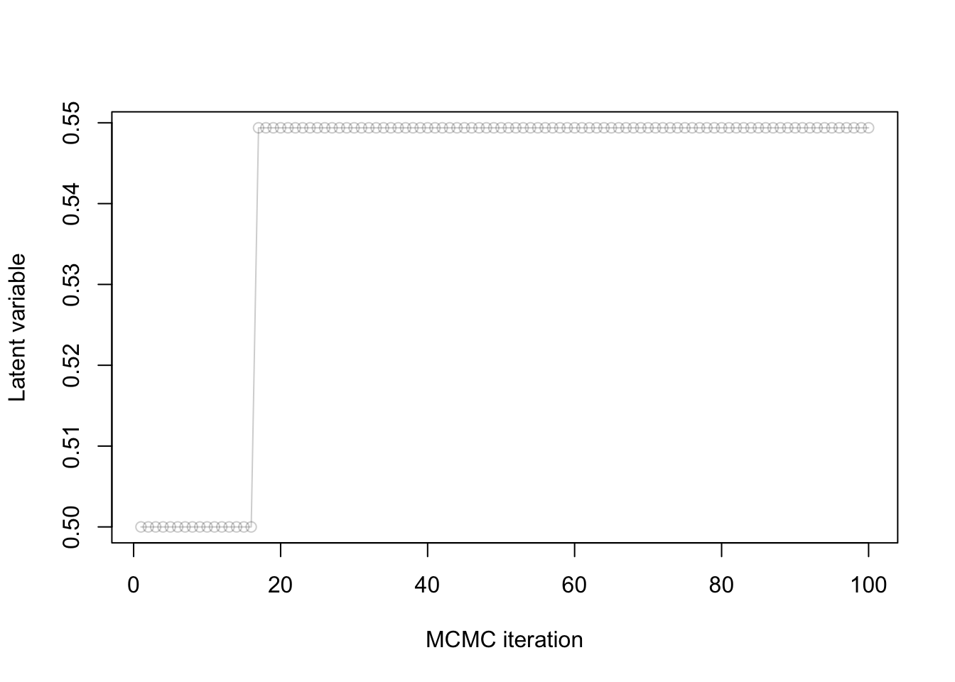
Is this chain mixing well?
Why or why not?
If it is not, what course of action do you recommend?

Click for answer

No.
Because the rejection rate is too high.
Decrease \(\sigma_p\).

Irreducibility

Consider the following MH setup:

\(\gamma(x) = \mathbb{1}[x \in \{1, 2, \dots, 10\}]\)
\(q(x' | x) = \mathbb{1}[x' \in \{x-1, x+1\}]/2\).

Define irreducibility.
Prove that the MH algorithm is irreducible in this setup.

Click for answer

See consistency of MH.
Let \(x, x' \in \{1, 2, \dots, 10\}\) (these are the only points where \(\gamma(x) > 0\)). Suppose first \(x' > x\) (the case \(x' < x\) is done similarly). Pick \(m = x' - x\), and note \[\begin{align*} \mathbb{P}(X^{(m)}= x' | X^{(0)} = x) &> \mathbb{P}(X^{(m)}= x', X^{(m-1)} = x'-1, X^{(m-2)} = x'-2, \dots, X^{(1)} = x+1 | X^{(0)} = x) \\ &= (1/2)^m > 0. \end{align*}\]

MCMC diagnostics

Explain how to detect slow mixing from a rank plot.

Click for answer

When one of the chains has a shape that deviates from the uniform distribution, we can raise a warning that there is slow mixing.

MCSE

How would you proceed if you want to decrease Monte Carlo Standard Error (MCSE)?

Click for answer

Increase the number of MCMC iterations.

Debugging

You wish to write Stan model for logistic regression with normal priors on the parameters with prior variance 100.

Consider the following draft of a Stan model:

data { 
  int N
  array[N] int y
}

model {
  slope ~ normal(0, 100);
  intercept ~ normal(0, 100);
  for (i in 1:N) {
    y[i] ~ bernoulli(inv_logit(intercept + slope * i));
  }
}

Identify as many bugs as you can, and correct each.

Click for answer

Missing declaration of the parameters:

parameters { 
  real slope;
  real intercept;
}

Missing two ; at the end of the lines in data.
The second argument of normal in Stan is a standard deviation, not a variance, so it should be slope ~ normal(0, 10);.
Similarly for the intercept.

The full correct code is taken from the clicker answers in the “hands on” page.

Effective sample size from asymptotic variance

Recall that the CLT for i.i.d. and Markov chains give us the following approximations:

\(\sqrt{M} (\bar X_\text{Markov} - \mu) \approx \sigma_a G,\)
\(\sqrt{n_e} (\bar X_\text{iid} - \mu) \approx \sigma G,\)

where \(M\) is the number of iterations, \(n_e\) is the effective sample size, \(\bar X_\text{Markov}\) and \(\bar X_\text{iid}\) are the MC estimators based on MCMC and i.i.d. sampling respectively, \(G\) is standard normal, \(\mu\), \(\sigma\) are the posterior mean and standard deviation, and \(\sigma_a\) is the asymptotic variance.

Use these two approximations to write a formula for the effective sample size based on \(\sigma\), \(\sigma_a\) and \(M\).

Click for answer

See lecture notes.

Independence: prior vs posterior

Suppose we place a prior where \(X_1\) and \(X_2\) are independent, say \(X_i \sim {\mathrm{Bern}}(0.5)\) independently. If we condition on some data \(Y\), will \(X_1\) and \(X_2\) always be independent under the posterior?

Click for answer

No. Consider for example \(Y = X_1 \text{ xor } X_2\), where recall that \(x \text{ xor } y\) iff exactly one of \(x_1, x_2\) is equal to one. Then under the posterior distribution that \((Y = 1)\), we have that \(X_1\) is completely determined by \(X_2\), i.e. \(\mathbb{P}(X_1 = x_1, X_2 = x_2 | Y = 1) \neq \mathbb{P}(X_1 = x_1 | Y = 1) \mathbb{P}(X_2 = x_2 | Y = 1)\). Many other counter examples are possible.

Footnotes

Where convergence is either almost sure (strong consistency), or in probability (weak consistency).↩︎

Outline

Topics

Important note

Libraries needed to run the example below

Model construction

Using the ~ notation

Rao-blackwellization

Model debugging

Normalization constant

Intervals

Bias and consistency

Stan-based prediction

Metropolis-Hastings

Stan

Reasoning about MH

Irreducibility

MCMC diagnostics

MCSE

Debugging

Effective sample size from asymptotic variance

Independence: prior vs posterior

Footnotes

Using the `~` notation