Censoring

Outline

Topics

• Recognizing censoring
• Modelling censoring

Rationale

Censoring is an example of a data collection process. We will see a case study where ignoring the data collection process literally cost many lives…

Example: Chernobyl, 1986

• In 1986, the Chernobyl Nuclear Power Plant exploded.
• Initially, the reactor crew chief, A. Akimov, assumed the core reactor was intact.

Data generation

• The numbers used in this page are synthetic but inspired by a true story.
• Let us not look at the data generating code just yet, we will come back to it.

set.seed(1)

# detection limit: value higher than that stay at the limit
limit = 1.1 

n_measurements = 10

true_mean = 5.6

# data, if we were able to observe perfectly
y = rexp(n_measurements, 1.0/true_mean)

# number of measurements higher than the detection limit
n_above_limit = sum(y >= limit)
n_below_limit = sum(y < limit)

# subset of the measurements that are below the limit:
data_below_limit = y[y < limit]

# measurements: those higher than the limit stay at the limit
measurements = ifelse(y < limit, y, limit)

Measuring radiation levels

• A dosimeter is a device measuring ionizing radiation.
  • Unit: roentgens per second (R/s).
• Suppose that:
  • If ionizing radiation is greater than 1.5 R/s \(\Rightarrow\) we think the reactor is breached (radiation coming out of the reactor core).
  • If ionizing radiation is smaller than 1.5 R/s \(\Rightarrow\) we think the reactor is not breached.
• We send 10 workers each with a dosimeter.
• The average over the 10 readings is:

mean(measurements)

[1] 1.012227

• All good?
• Let us look at the raw data and histogram.

suppressPackageStartupMessages(library("ggplot2"))
df = data.frame(measurements = measurements)

ggplot(df, aes(x = measurements)) +
  geom_histogram() + 
  geom_rug(alpha = 0.1) + 
  theme_minimal()

measurements

 [1] 1.1000000 1.1000000 0.8159577 0.7828535 1.1000000 1.1000000 1.1000000
 [8] 1.1000000 1.1000000 0.8234575

Question: is this concerning?

Click for choices

1. No concerns, all good. Let’s go in the reactor to inspect.
   
2. It is unusual that there are many repeated measured values, but this can happen when measuring discrete distributions.
3. It is unusual that there are many repeated measured values, this is due to high noise.
4. It is concerning that there are repeated measured values, this could be due to the dosimeters having a detection limit.
5. None of the above.

Click for answer

The correct answer is 4: dosimeters can suffer from a saturation effect, i.e. if the radiation is stronger than the detection limit, the measurement can underestimate the true value (potentially by a huge amount).

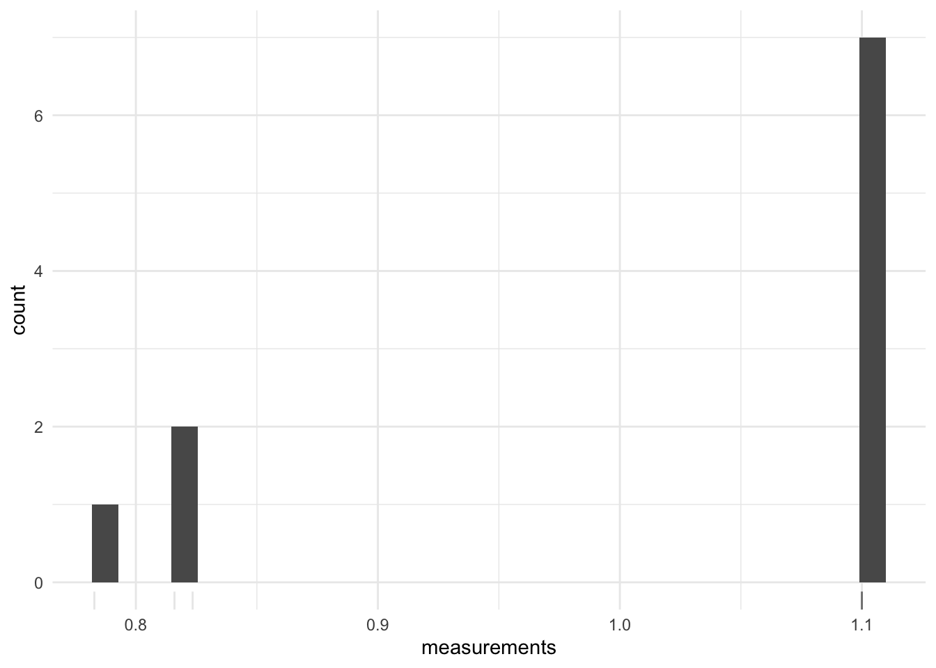
Sadly, in reality the reactor crew chief A. Akimov picked option 1. In reality, the effect was even more extreme: the detection limit of the dosimeters available was 0.001 R/s whereas in the worst hit region the true value was round 5.6 R/s. A lethal dose is around 500 R.

A. Akimov and his crew went in the reactor. Most, including Akimov, died from radiation exposure within 3 weeks.

Go back to the generating code, Section 2.1, to see how I generated the data.

Bayesian approach to censoring

• What we have encountered in the Chernobyl example is known as censoring.
• Solution: modelling the censoring process.

Mathematical description

• Let \(L\) denote a detection limit (here \(L = 1.1\))
• Let \(X\) denote the unknown parameter.
• Let \(i\) denote the observation index (worker \(i \in \{1, 2, \dots, 10\}\) in our example)
• Let \(H_i\) denote the measurements before censoring (i.e., if we had a perfect measurement device immune to saturation effects).
• Let \(C_i\) denote a binary indicator on the censoring (i.e., equal to one if the imperfect device has a saturation, zero otherwise).
• Let \(Y_i = C_i L + (1 - C_i) H_i\).

In the Chernobyl example, we will use the following model:

\[\begin{align*} X &\sim {\mathrm{Exp}}(1/100) \\ H_i &\sim {\mathrm{Exp}}(X) \\ C_i &= \mathbb{1}[H_i \ge L], \\ Y_i &= C_i L + (1 - C_i) H_i. \end{align*}\]

The goal is to compute \(\mathbb{E}[\text{mean parameter of uncensored measurements} | Y] = \mathbb{E}[1/X | Y]\).

Stan implementation

suppressPackageStartupMessages(library(cmdstanr))

chernobyl_naive.stan

data {
1  int<lower=0> n_above_limit; //
2  int<lower=0> n_below_limit; //
  real<lower=0> limit;
3  vector<upper=limit>[n_below_limit] data_below_limit; //
  
}

parameters {
  real<lower=0> rate; 
4  vector<lower=limit>[n_above_limit] data_above_limit; //
}

model {
  // prior
  rate ~ exponential(1.0/100);
  
  // likelihood
  data_above_limit ~ exponential(rate);
  data_below_limit ~ exponential(rate); 
}

generated quantities {
  real mean = 1.0/rate;
}

1

The number of \(H_i\)’s above the detection limit.

2

The number of \(H_i\)’s below the detection limit.

3

The \(H_i\)’s below the limit are observed, so they go in the data block.

4

The \(H_i\)’s above the limit are not observed, so they go in the parameters block (a better name would have been “latent block”).

mod = cmdstan_model("chernobyl_naive.stan")
fit = mod$sample(
  seed = 1,
  chains = 1,
  data = list(
            limit = limit,
            n_above_limit = n_above_limit, 
            n_below_limit = n_below_limit,
            data_below_limit = data_below_limit
          ),  
  output_dir = "stan_out",
  refresh = 10000,
  iter_sampling = 100000                   
)

Running MCMC with 1 chain...

Chain 1 Iteration:      1 / 101000 [  0%]  (Warmup) 
Chain 1 Iteration:   1001 / 101000 [  0%]  (Sampling) 
Chain 1 Iteration:  11000 / 101000 [ 10%]  (Sampling) 
Chain 1 Iteration:  21000 / 101000 [ 20%]  (Sampling) 
Chain 1 Iteration:  31000 / 101000 [ 30%]  (Sampling) 
Chain 1 Iteration:  41000 / 101000 [ 40%]  (Sampling) 
Chain 1 Iteration:  51000 / 101000 [ 50%]  (Sampling) 
Chain 1 Iteration:  61000 / 101000 [ 60%]  (Sampling) 
Chain 1 Iteration:  71000 / 101000 [ 70%]  (Sampling) 
Chain 1 Iteration:  81000 / 101000 [ 80%]  (Sampling) 
Chain 1 Iteration:  91000 / 101000 [ 90%]  (Sampling) 
Chain 1 Iteration: 101000 / 101000 [100%]  (Sampling) 
Chain 1 finished in 1.6 seconds.

fit$summary(NULL, c("mean", "mcse_mean"))

# A tibble: 10 × 3
   variable               mean mcse_mean
   <chr>                 <dbl>     <dbl>
 1 lp__                -19.3    0.0123  
 2 rate                  0.393  0.000927
 3 data_above_limit[1]   4.54   0.0249  
 4 data_above_limit[2]   4.52   0.0244  
 5 data_above_limit[3]   4.49   0.0236  
 6 data_above_limit[4]   4.51   0.0214  
 7 data_above_limit[5]   4.48   0.0260  
 8 data_above_limit[6]   4.53   0.0234  
 9 data_above_limit[7]   4.52   0.0243  
10 mean                  3.41   0.0178  

suppressPackageStartupMessages(library(bayesplot))
suppressPackageStartupMessages(library(ggplot2))
mcmc_areas_ridges(fit$draws("mean")) + 
  theme_minimal() + 
  scale_x_continuous(limits = c(0, 10)) 

Back to the question of whether the radiation is greater than 1.5 R/s:

samples = as.vector(fit$draws("mean"))

sum(samples > 1.5) / length(samples)

[1] 0.90655