Laplace approximation

Outline

Topics

• Laplace: an approximation to the posterior motivated by BvM.
• Example of Laplace’s failure modes.

Rationale

Laplace approximation is a useful tool for some (but not all) Bayesian models. The Laplace approximation is attractive because it is sometimes very cheap to compute and accurate. Understanding that approximation will also help understand the BvM theorem introduced in the previous page.

Laplace approximation: input and output

Input: an un-normalized density \(\gamma(x)\), where \(x\) is real-valued (or vector valued).

Output: an approximation \(q(x)\) for \(\gamma\) for which the normalization constant can be computed easily.

Think about it as an alternative to SNIS.

Example

We use the same example as this week’s lab:

\[\begin{align*} X &\sim {\mathrm{Unif}}(0, 1) \\ Y|X &\sim {\mathrm{Binom}}(n, X). \end{align*}\]

We have implemented \(\gamma(x) = p(x, y)\) for this model in R, in a function called lab5logdensity.

lab5logdensity = function(x) {
  ifelse(x < 0 | x > 1, -Inf, dbinom(n_successes, size = n_trials, prob = x, log = TRUE))
}

# we will also need a utility to maximize a function and get the second derivative at the optimum
maximize = function(objective, start = 0.5) {
  res = nlm(f = function(x) -objective(x), start, hessian = TRUE) 
  # the negative signs here is because nlm minimizes, so we negated the objective, we convert back below...
  list(
    max = -res$minimum,
    argmax = res$estimate, 
    second_derivative = -res$hessian
  )
}

n_trials = 800
n_successes = 0.8 * n_trials

Since we study the big data regime, we set the number of data points fairly large:

n_trials

[1] 800

The observed data \(y\) is:

n_successes 

[1] 640

In the real world, we would not need the Laplace here since we know the posterior is a Beta distribution (by conjugacy, covered in the lab this week). But in real problems, it is rare that you can use conjugacy calculation, it is a fragile property.

Motivation

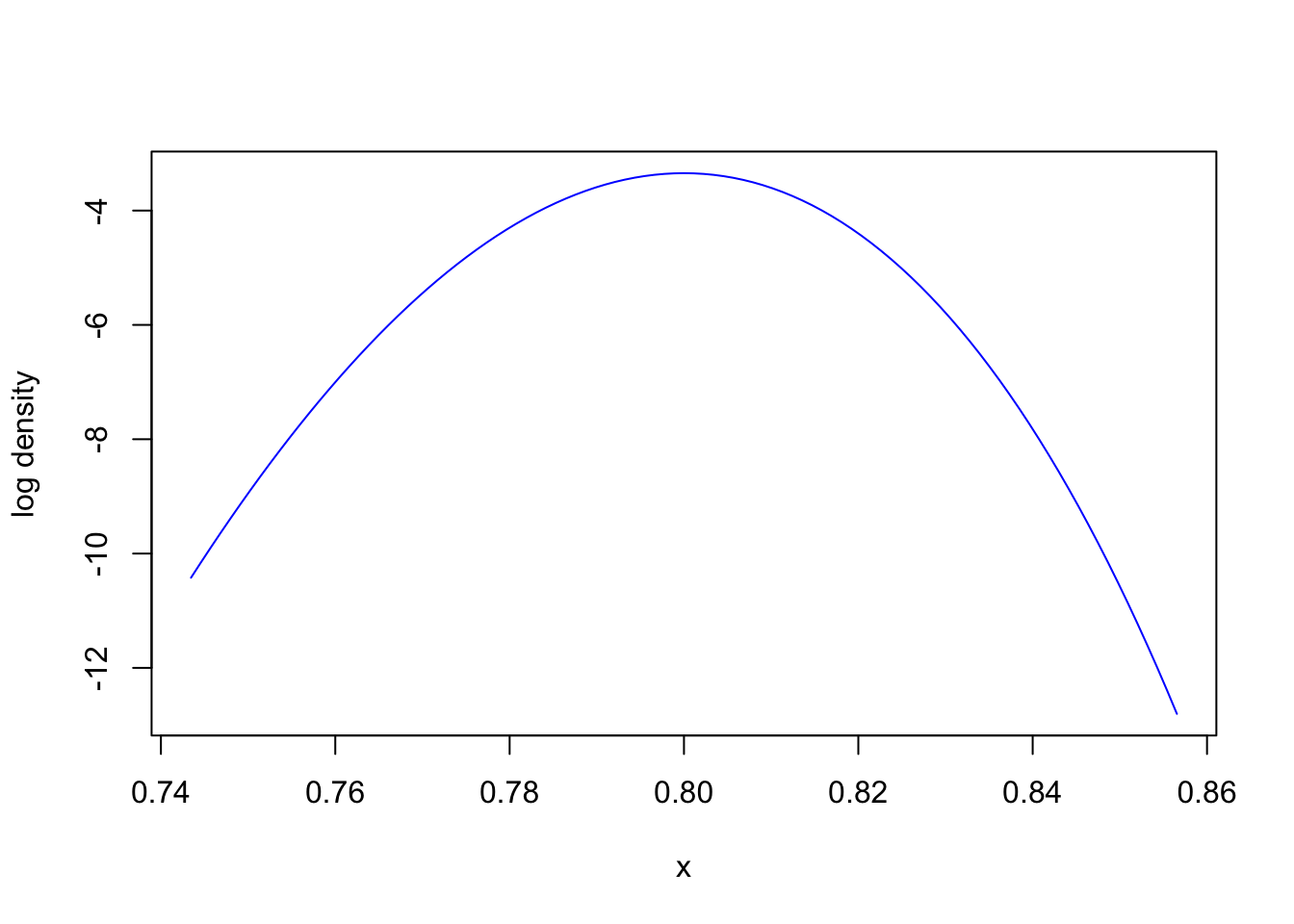
Let us look at the log density near the mode of the posterior:¹

opt = maximize(lab5logdensity, 0.5)

second_derivative = opt$second_derivative
zoomed_width = 4 / sqrt(-second_derivative)
center = opt$argmax 
left = center - zoomed_width
right = center + zoomed_width

curve(lab5logdensity, from = left, to = right, col = "blue", ylab = "log density")

Question: How would you approximate such a function?

Click for answer

A quadratic function seems a good candidate.

Specifically, a common way to do so is to do a Taylor expansion up to the second degree polynomial, centered at the mode.

Why the mode? For regular targets, this is where most of the posterior mass is concentrated (as shown in the lab this week). So we want our approximation to be good around the mode.

Taylor expansion

Notation: denote the function above by \(\ell(x) = \log \gamma(x)\).

Notation: denote the MAP (i.e., \(\operatorname{arg\,max}\ell\)) by \(\hat x\).

Recall Taylor’s theorem (shown here for the second order):

\[\ell(x) = \ell(\hat x) + \ell'(\hat x) (x - \hat x) + \frac{\ell''(\hat x)}{2!}(x - \hat x)^2 + R(x),\] where different flavours of Taylor’s theorem will give different types of control of the residual error term \(R(x)\) (we will not go into that level of detail today).

Question: one term in the Taylor expansion is zero. Which one? Why?

Click for answer

The second term is zero, since \(\ell'(\hat x) = 0\). This is because \(\hat x\) is the location of the maximum. Hence assuming that \(\hat x\) is an interior point, the derivative at this point is zero.

So removing the zero term and ignoring the residual, we obtain the Laplace approximation:

\[ \ell(x) \approx \ell(\hat x) + \frac{\ell''(\hat x)}{2}(x - \hat x)^2. \]

Implementation

All the ingredients in the Taylor approximation can be obtained using an optimizer package. For the second derivative, either automatic differentiation or finite differences can be used.

Here is a simple implementation:

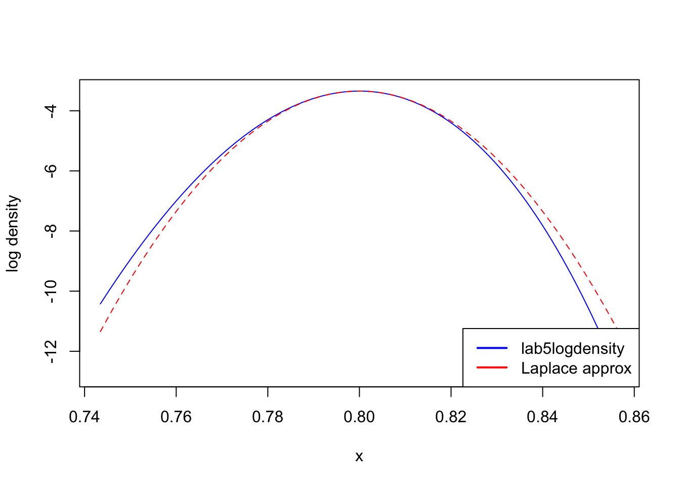
laplace_approx = function(opt) {
  
  x_hat = opt$argmax
  maximum = opt$max
  second_derivative = opt$second_derivative
  
  approx = function(x) {
    return(maximum + second_derivative / 2 * (x - x_hat)^2)
  }
  
  return(approx)
}

laplace = laplace_approx(opt)

curve(lab5logdensity, from = left, to = right, col = "blue", ylab = "log density")
curve(laplace, from = left, to = right, add = TRUE, col = "red", lty = 2)

legend(
  "bottomright",
  legend = c("lab5logdensity", "Laplace approx"),
  col = c("blue", "red"),
  lwd = 2
)

As you can see, the approximation is quite good where it matters (near the mode)!

Let us denote the Laplace approximation by \(\log q\):

\[ \ell(x) \approx \underbrace{\ell(\hat x) + \frac{\ell''(\hat x)}{2}(x - \hat x)^2}_{\log q(x)}. \]

Question: can you interpret \(q(x)\) as a density?

Click for Hint

• Take the \(\exp\).
• Ignore multiplicative constants that do not depend on \(x\).

Click for choices

1. Normal with mean \(\hat x\) and variance \(\ell''(\hat x) / 2\)
2. Normal with mean \(\hat x\) and variance \(-1/\ell''(\hat x)\)
3. Exponential with rate \(\ell''(\hat x)\).
4. Exponential with rate \(\ell(\hat x)\).
5. None of the above.

Click for answer

We know by construction that the log density is a quadratic function. This characterizes normal densities.

Now let us obtain the mean and variance parameters of that normal…

After exponentiation:

\[\begin{align*} q(x) &= \exp\left(\ell(\hat x) + \frac{\ell''(\hat x)}{2}(x - \hat x)^2\right) \\ &\propto \exp\left(\frac{\ell''(\hat x)}{2}(x - \hat x)^2\right). \end{align*}\]

Hence we have to match the above with the parametrization of a normal, given by:

\[\text{constant} \times \exp\left( - \frac{(x - \mu)^2}{2\sigma^2}\right).\]

Hence we have \(\mu = \hat x\) and \(\sigma^2 = -1/\ell''(\hat x)\).

Now what is that constant? The painful way to find it would be to use the fact that a density should integrate to one, and to compute:

\[\int \exp\left( - \frac{(x - \mu)^2}{2\sigma^2}\right) \mathrm{d}x = 1/\text{constant}.\]

But there is a shortcut!

The key ingredient of the shortcut is (the proof of it is reviewed in the lab this week):

Proposition: if two densities are proportional, \(f_1 \propto f_2\) then they are equal, \(f_1 = f_2\).

So since we know that \(q\) is proportional to a normal, it is a normal, and so that means we can look at wikipedia page to get the value of that constant. You will find it is \(1/\sqrt{2\pi\sigma^2}\). In other words, someone solved the above integral for you (and that’s good because that integral is tricky to work out!).

Asymptotic analysis of Laplace’s approximation quality

• Consider the same setup as BvM (increasing random datasets).
• Denote the variance of the Laplace approximation computed from \(Y_{1:n}\) by \(\sigma^2_n\).
• Recall that the asymptotic normal distribution in BvM had variance \(-I_n^{-1}\).

Note: \(\lim_{n\to\infty} \sigma^2_n / (-I_n^{-1}) = 1\).

To see why, notice that the second derivative of \(\ell\) is the sum of the prior’s second derivative at \(\hat x\), denoted \(-S = (\log p)''(\hat x)\), and the observed information \(-I_n\): \[\begin{align*} \log \gamma(x) &= \log p(x, y) \\ &= \log p(x) p(y|x) \\ &= \log p(x) + \log p(y | x), \\ \Longrightarrow \underbrace{\frac{\partial^2}{\partial x^2} \log \gamma(x) }_{\ell''(x)} &= \underbrace{\frac{\partial^2}{\partial x^2} \log p(x)}_{-S} + \underbrace{\frac{\partial^2}{\partial x^2} \log p(Y_{1:n} | x)}_{\to -I_n}. \end{align*}\]

hence

\[ \lim \frac{\sigma^2_n}{-I_n^{-1}} = \lim \frac{I_n}{S + I_n} = \lim \frac{\frac{1}{n} I_n}{\frac{1}{n} S + \frac{1}{n} I_n}. \] Finally, \(\frac{1}{n}S\) converges to zero, while by the law of large numbers, \(\frac{1}{n} I_n\) converges to a constant, namely the Fisher information, \(\mathbb{E}[I_n]\).

Conclusion:

• The Laplace approximation converges to the same normal as the one appearing in BvM.
• Hence, when BvM applies, the Laplace approximation also gets arbitrarily accurate as \(n \to \infty\).

Estimating expectation from a Laplace approximation

Option 1: for some test functions \(g\), you can use known expression from the normal (e.g. to compute posterior mean, variance).

Option 2: use simple Monte Carlo, where the i.i.d. samples come from the Laplace approximation.

Option 3: use the Laplace approximation as a proposal in SNIS.

With SNIS+Laplace, even for finite \(n\), the error in the Laplace approximation gets corrected in the large \(M\) regime.

Multivariate version

The second derivative is simply replaced by the Hessian matrix \(M\) at \(\hat x\),

\[q(x) = \mathcal{N}(\text{mean} = \hat x, \text{covariance matrix} = -M^{-1}),\]

where

\[M_{i,j} = \frac{\partial^2}{\partial x_i \partial x_j} \log \gamma(x)\Bigg|_{\hat x}.\]

Typical failure mode

Consider the following model:

\[\begin{align*} X_1 &\sim {\mathrm{Unif}}(0, 1) \\ X_2 &\sim {\mathrm{Unif}}(0, 1) \\ X &= X_1 X_2 \\ Y|X_1, X_2 &\sim {\mathrm{Binom}}(n, X). \end{align*}\]

Let us use simPPLe to approximate the posterior given a fairly large number of observations (\(n = 800\)):

source("../../solutions/simple.R")
source("../blocks/simple_utils.R")

unid_size = 800

unidentifiable = function() {
  x1 = simulate(Unif(0, 1))
  x2 = simulate(Unif(0, 1)) 
  x = x1 * x2
  observe(unid_size / 8, Binom(unid_size, x)) 
  return(c(x1, x2))
}

posterior = posterior_particles(unidentifiable, 10000)
weighted_scatter_plot(posterior, plot_options = list(xlab="x1", ylab="x2"))

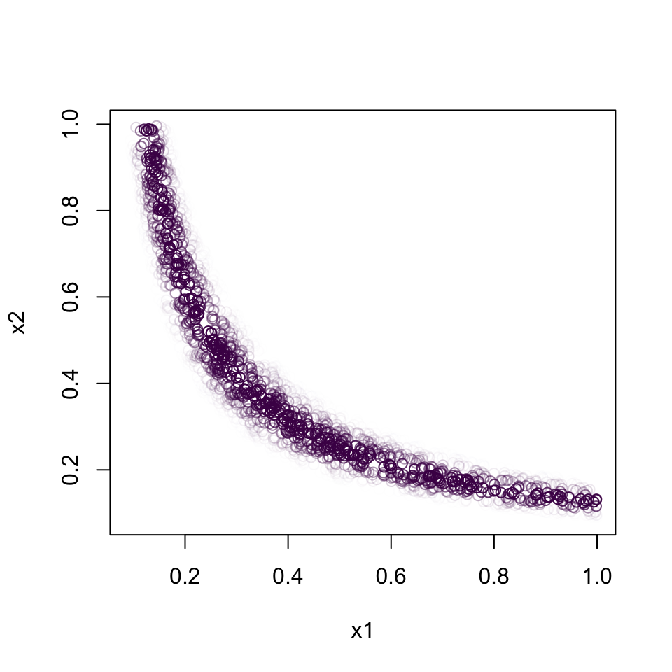
• In 2 dimensions, the Laplace approximation is a bivariate normal.
• Hence the contour lines of Laplace approximations are restricted to ellipses.
• This means that the Laplace approximation would be very poor here.

Question: which of BvM’s key assumptions is violated here?

Footnotes

1. Why taking the log? Superficially, we will see in this example that this makes the density function easier to approximate. Other transforms may work better in specific cases, but there is a deeper reason connected to BvM covered in this page. Roughly, the log is special because it changes products into sums. The products come from chain rule of probability, and turning them into sums will let the law of large number and central limit theorem kick in, which are theorems about sums.