suppressPackageStartupMessages(library(cmdstanr))
suppressPackageStartupMessages(library(ggplot2))
suppressPackageStartupMessages(library(dplyr))
suppressPackageStartupMessages(library(bayesplot))

data = read.csv(url("https://github.com/UBC-Stat-ML/web447/raw/main/data/ScoreData.csv"))
mod = cmdstan_model("../w10_modelling/students_guessing.stan")VI with Stan
Outline
Topics
- Calling VI with cmdstanr
- Main options
- Interpreting the output
- Alternatives to Stan
Rationale
Now that you know how to write Stan models, we see here that you can run not only HMC but also VI.
Example
We will use the model for detecting random guessing and compare the output of variational inference and HMC.
Calling VI with cmdstanr
The commands are very similar to how we call HMC.
First create the model exactly as before:
Then to run VI:
- 1
-
This specifies the variational family \(\mathscr{Q}\). Use
meanfieldfor a normal with diagonal covariance,fullrankfor any normal. - 2
- How many samples from \(q^*\) to output.
------------------------------------------------------------
EXPERIMENTAL ALGORITHM:
  This procedure has not been thoroughly tested and may be unstable
  or buggy. The interface is subject to change.
------------------------------------------------------------
Gradient evaluation took 5.6e-05 seconds
1000 transitions using 10 leapfrog steps per transition would take 0.56 seconds.
Adjust your expectations accordingly!
Begin eta adaptation.
Iteration:   1 / 250 [  0%]  (Adaptation)
Iteration:  50 / 250 [ 20%]  (Adaptation)
Iteration: 100 / 250 [ 40%]  (Adaptation)
Iteration: 150 / 250 [ 60%]  (Adaptation)
Iteration: 200 / 250 [ 80%]  (Adaptation)
Success! Found best value [eta = 1] earlier than expected.
Begin stochastic gradient ascent.
  iter             ELBO   delta_ELBO_mean   delta_ELBO_med   notes
   100          -88.203             1.000            1.000
   200          -87.428             0.504            1.000
   300          -86.567             0.340            0.010   MEDIAN ELBO CONVERGED
Drawing a sample of size 1000 from the approximate posterior...
COMPLETED.
Finished in  0.1 seconds.
Note: calling mod$variational does two things:
- First, find \(q^* \in \mathscr{Q}\) that is closest to \(\pi\).
- Sample from \(q^*\)
output_samplestimes (this provides independent and identical samples).
Compare this to how we ran HMC:
fit.hmc = mod$sample(
  seed = 1,
  refresh = 500,
  output_dir = "stan_out",
  chains = 1,
  data = list(
            n_students = length(data$Score),
            scores = data$Score
          )
)
Running MCMC with 1 chain...
Chain 1 Iteration: 1 / 2000 [ 0%] (Warmup)
Chain 1 Iteration: 500 / 2000 [ 25%] (Warmup)
Chain 1 Iteration: 1000 / 2000 [ 50%] (Warmup)
Chain 1 Iteration: 1001 / 2000 [ 50%] (Sampling)
Chain 1 Iteration: 1500 / 2000 [ 75%] (Sampling)
Chain 1 Iteration: 2000 / 2000 [100%] (Sampling)
Chain 1 finished in 0.4 seconds.Warning: 1 of 1 chains had an E-BFMI less than 0.3.
See https://mc-stan.org/misc/warnings for details.Comparing the output of VI and HMC
Recall that in the mixture page we defined random variables \(X_i = \mathbb{E}[G_i | A_i, Y]\), the “guessing probabilities”, with support on \([0, 1]\).
Let us look at the posteriors of \(X_i\) for HMC vs VI:
Code
library(bayesplot)
library(ggplot2)
library(dplyr)
library(latex2exp)

vars = fit.hmc$metadata()$model_params
sel  = grep("^guessing_probabilities.*", vars, value = TRUE)

data_hmc = mcmc_intervals_data(fit.hmc$draws(variables = sel)) %>%
  mutate(method = "HMC")

data_vi = mcmc_intervals_data(fit.variational$draws(variables = sel)) %>%
  mutate(method = "Variational")

bind_rows(data_hmc, data_vi) %>%
  ggplot(aes(x = m, y = parameter, color = method)) +
  geom_linerange(aes(xmin = ll, xmax = hh),
                 position = position_dodge(width = 0.5)) +
  geom_linerange(aes(xmin = l, xmax = h),
                 position = position_dodge(width = 0.5), size = 1.5) +
  geom_point(position = position_dodge(width = 0.5), size = 2) +
  scale_x_continuous(limits = c(0, 1)) +
  theme_minimal() +
  labs(
    x = TeX("$X_i$"),
    y = NULL,
    color = "Method"
  )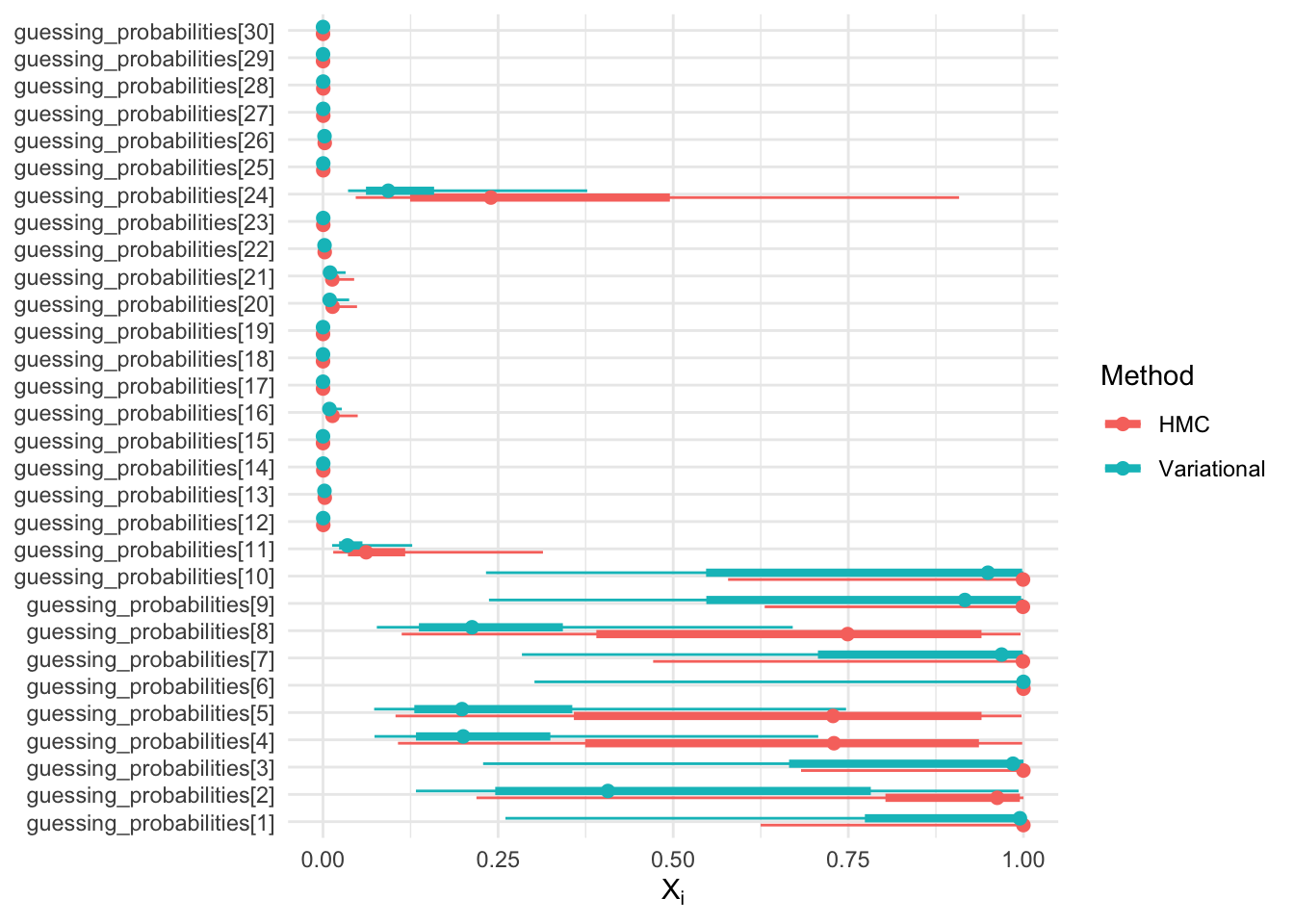
Question: If the variational family is normal, how come the support of \(X_i\) seems to be contained in the interval \([0, 1]\)?
CautionClick for choices
- The support of the normal distribution can be adjusted to be [0, 1]
- The variational fit is done in the unconstrained space
- Stan discards all samples that violate the support constraints
- The support is not actually contained in the interval [0, 1]
- None of the above
CautionClick for answer
Correct answer is: the variational fit is done in the unconstrained space.
As discussed earlier, Stan uses a change of variable to transform the latent variables into an unconstrained space. This is the same technique as used in exercise 6.
In exercise 6 we called the constraining transform \(c\).
This means that after sampling \(\tilde X^{(m)} \sim q^*\), Stan will transform it back to the constrained (original) parameterization, i.e., \(X^{(m)} = c^{-1}(\tilde X^{(m)})\).
The samples in the fit objects are the independent and identically distributed random variables \(X^{(1)}, \dots, X^{(M)}\).
Alternatives
- Stan supports another Variational method, “path finder”, which is often faster.
- But neither path finder nor Stan VI support data subsampling, so for large dataset, consider using NumPyro.